1
Stochastic Modular Robotic Systems: A Study of Fluidic Assembly Strategies Michael T. Tolley, Member, IEEE, Michael Kalontarov, Jonas Neubert, Member, IEEE, David Erickson, and Hod Lipson, Member, IEEE Abstract—Modular robotic systems typically assemble using deterministic processes where modules are directly placed into their target position. By contrast, stochastic modular robots take advantage of ambient environmental energy for the transportation and delivery of robot components to target locations, thus offering potential scalability. The inability to precisely predict component availability and assembly rates is a key challenge for planning in such environments. Here, we describe a computationally efficient simulator to model a modular robotic system that assembles in a stochastic fluid environment. This simulator allows us to address the challenge of planning for stochastic assembly by testing a series of potential strategies. We first calibrate the simulator using both high-fidelity computational fluiddynamics simulations and physical experiments. We then use this simulator to study the effects of various system parameters and assembly strategies on the speed and accuracy of assembly of topologically different target structures. Index Terms—Biologically inspired robots, cellular and modular robots, fluidic assembly, stochastic robotics.
I. I. INTRODUCTION
M
ODULAR self-reconfigurable robotic systems have the potential to adapt to new environments and tasks by changing the connectivity of their constituent modules to transform their morphology [1], [2]. This capability could result in a versatile system that can accomplish unforeseen goals, repair itself when damaged, efficiently reuse components, and self-replicate. These remarkable advantages, howManuscript received May 28, 2009; revised December 8, 2009, February 9, 2010, and March 25, 2010; accepted March 25, 2010. Date of publication May 10, 2010; date of current version June 9, 2010. This paper was recommended for publication by Associate Editor A. Ijspeert and Editor L. Parker upon evaluation of the reviewers’ comments. This work was supported by the Defense Advanced Research Projects Agency Defense Science Office Programmable Matter Program under Grant W911NF-08-1-0140 and the U.S. National Science Foundation’s Office of Emerging Frontiers in Research and Innovation under Grant 0735953. The work of M. T. Tolley was supported by the Natural Sciences and Engineering Research Council of Canada through the Postgraduate Scholarship Program. M. T. Tolley, J. Neubert, and H. Lipson are with the Computational Synthesis Laboratory, Cornell University, Ithaca, NY 14853 USA (e-mail:
[email protected];
[email protected];
[email protected]). M. Kalontarov and D. Erickson are with the Integrated Micro- and Nanofluidic Systems Laboratory, Cornell University, Ithaca, NY 14853 USA (email:
[email protected];
[email protected]). This paper has supplementary downloadable material available at htttp://ieeexplore.ieee.org. provided by the author. The material includes one video. The size is 28.2 MB. Contact
[email protected] for further questions about this work. Color versions of one or more of the figures in this paper are available online at http://ieeexplore.ieee.org. Digital Object Identifier 10.1109/TRO.2010.2047299
ever, come with severe challenges in the mechanical design and control of the system and its modules. Previous work on modular selfreconfigurable robot systems has addressed many of these challenges: A variety of system designs have been proposed, including mobile modules with chain [3]–[6] and planar or 3-D lattice [7]–[9] connectivity. Such approaches require complex mechanisms and high energy budgets that are difficult to scale to small dimensions and large numbers. An alternative approach sidesteps the demands of module locomotion by allowing the modules to move freely in a stochastic environment and by controlling the connectivity only when modules come into contact [9] –[14]. This biologically inspired stochastic assembly approach forms the basis of the work presented here. The type of control required for a modular robotic system depends heavily on its architecture. Many of the systems with mobile modules assemble and reconfigure themselves with both low (module)-level and high (system)-level control [15],[16]. Stochastic assembly systems avoid the requirements for complex motion -planning control at the module level and instead require only a decision of whether or not to connect two components when they come into contact. This decision may either be made based on local information (which is similar to cellular automata) or made centrally and distributed via intercomponent communication. However, since the arrival time of a component at any given location cannot be predicted deterministically, robust assembly strategies must be employed to account for these uncertainties and accelerate assembly/reconfiguration. Thus, in addition to simplifying module design, a stochastic assembly approach simplifies modulelevel control requirements, at the cost of increased uncertainty that must be compensated for in the system-level control scheme. Previous work has examined various aspects of the design and control of robotic stochastic assembly systems. Inspired by the self-assembly research [16],[18] these systems generally add the ability to control their configurations on the fly. White et al. [13] first demonstrated the stochastic selfassembly and reconfiguration of triangular modules on an air table and suggested that simple assembly strategies could lead to dramatically different scalability. These principles were then repeated in 3-D [14],[18]. Griffith et al. [9] demonstrated the selfreplication of a 2-D template string from electrome-
2 chanical parts moving about stochastically on an air table. When the parts come into contact, they latch together, communicate with one another, and decide whether to disengage the latches. Klavins [11] designed a similar 2-D system of ―programmable parts‖ along with a method of modeling the connectivity of these parts using graph grammars. A control scheme was also proposed in which the various interactions are viewed as chemical reactions with parameters that can be tweaked to achieve desired target structures. Gilpin et al. [12] have taken alternative selfdisassembling approach that begins with a lattice of modules that communicate and establish connectivity as required to form a desired structure while unnecessary components are released stochastically. In previous work, we have demonstrated the assembly of 2D structures from 500-μm-scale silicon components in a fluidic environment [18]. These components had a passive latching mechanism and assembled deterministically into arbitrarily defined structures with open- and closed-loop fluid control. We have also previously demonstrated experimental 3-D assembly from robotic cube-shaped modules in a fluidic environment [14]. However, the relatively large scale of this system (10 cm) led to slow assembly rates and made it difficult to demonstrate the experimental assembly of more than few components. This experimental work was complemented by a basic 3-D simulator that was used to examine some aspects of 3-D stochastic assembly. This simulator, however, included no fluidic forces. One of the major challenges in self-reconfigurable modular robotics has been scaling up the number of modules. The capability of a modular robotic system to realize its advantages over traditional systems is based largely on its ability to assemble large numbers of components with a fine resolution; however, systems composed of more than ∼50 modules have yet to be demonstrated [1]. In order to increase the resolution of current systems, it will be necessary to further reduce their modules’ sizes. Despite the reduction in module complexity due to stochastic assembly approaches, current limitations of microfabrication technologies (e.g., their 2-D nature) make the manufacture of 3-D robotic modules a difficult problem. Nonetheless, we believe that it should be possible to reduce all of the necessary components of a modular robotic system based on our fluidic assembly approach to fit inside a 1-cm cube. For this reason, we aim to develop a system of stochastic, Fluidically assembled modules of this scale. In this paper, we present a custom 3-D simulator to support this experimental effort. While a simulator is no substitute for a physical system, it does enable us to explore the large space of possible system parameters and assembly strategies much more efficiently. The challenge with solving mixed fluid–rigid -body systems is the high cost of computation. Our goal here is to make sufficient simplifications to make the problem tractable while still obtaining meaningful results. In order to gain
confidence in our simulator, we compare its results with those of a commercial computational fluid dynamics (CFD) package and with experimental results for specific test cases. We then use the simulation to examine the effects of different system parameters on assembly dynamics and explore various assembly strategies. Based on these results, we recommend system parameters for a fluidic assembly system and suggest a number of potential assembly strategies. We further discuss the tradeoffs between the various assembly strategies and the ramifications of these results for the design of achievable target structures. II. FLUIDIC SELF-ASSEMBLY CONCEPT At small scales, biological structures assemble themselves primarily in fluidic environment taking advantage of random Brownian motion as a component transportation mechanism. Inspired by this example, our approach to self-reconfigurable modular robotics involves unpowered cubes that rely on ambient stochastic fluid motion for transportation [14], [18]. Fluidic forces are additionally used to accelerate assembly by attracting cubes to where they are needed. Finally, a bonding force is used to hold the cubes together in the final structure. Structure formation begins by opening a sink on a growth substrate in order to attract nearby cubes (see Fig. 1). When a cube falls within the basin of attraction of the sink, it is pulled toward the sink where geometric interactions cause it to align with the growth substrate and a bonding mechanism activates to hold the cube in place. Once attached, the cube is able to
Fig. 1. Fluidic Self-Assembly Concept. (a) Fluid flow (which is indicated by arrows) into a substrate attracts a nearby module. (b) Once a module passes within close proximity of the target location, near-field forces (e.g., magnets) cause the module to align and attach. (c) Once attached, the module draws power from the substrate to activate on-board valves and redirect fluid flow through internal channels, thereby (d) attracting new modules at desired locations. This process continues layer-by-layer until the structure is complete.
3
(a)
(b)
Fig. 2. Stochastic fluidic assembly simulator. (a) To achieve computationally efficient simulation of our modular robotic system, we wrote a custom simulator in C++ using the ODE libraries. (b) Simplified fluidic forces were added to the ODE rigid-body simulation to model the forces applied to the modules. A module is shown here transparent with arrows representing these forces. The arrow labeled Fs,c represents the force exerted on the module by fluid exiting the assembly tank through the open sink (which is represented by a dark square). Fd is the fluid drag force resisting the motion of the cube. is a normal to the sink, and r is a vector from the sink to the cube.
draw power from the substrate to activate internal valves, thereby closing off internal channels as required to connect the bonded face with any number of exposed faces. This effectively moves the sink from its original location to one or more surfaces of the attached cube to attract new cubes to these locations. The target system is thus ―grown‖ by repeatedly opening sinks and by attracting and bonding cubes. Reconfiguration is achieved by deactivating the bonds to unwanted modules and allowing ambient fluid motion to carry them away while attracting components to new locations as required. III. SIMULATION As mentioned in Section I, the goal of this study was to develop a computationally efficient simulator to aid in the design and operation of a system based on the stochastic fluidic assembly concept, which is described in the previous section. Specifically, our goal was to develop a simulator that is capable of predicting the assembly rates and completion percentages for an arbitrary structure using various assembly approaches and system parameters. During the experimental system design phase, a simulator allows the exploration of various system parameters to inform the design and avoid unnecessary iterations. Additionally, even after completion of the experimental system, an accurate simulator allows experimentation with strategies and scenarios that would be impossible or too costly to test physically. A. Choice of Simulation Method In order to achieve our goals, we required a simulator that was as accurate as possible while maintaining computational efficiency. Using a full CFD simulation coupled with a rigid body solver would have been the most accurate approach to predicting the motion of the components in the assembly tank. However, this approach would also have been prohibitively expensive. For example, simulations of the motion of a single cube approaching a sink from a distance of two cube lengths
using the CFD software FLOW-3D (see Section III-C) took approximately 4.8 h to solve. Our initial goal was to simulate the assembly of a structure composed of approximately 100 cubes and to repeat the simulation for many different parameters and assembly strategies. Even with many computers working in parallel, it was apparent that CFD simulations would not be a tractable option. We thus decided to develop a simulation that would capture the assembly dynamics of the system without getting lost in the details of solving the fluid flow. We wrote our fluidic assembly system simulator [see Fig. 2(a)] in C++, using the Open Dynamics Engine [22] (ODE)— a stable, open-source, adaptable, computationally efficient rigid-body solver—for simulation of cube motion and collision detection. We then added simplified fluidic forces to model the effects of agitation and fluid drag, as well as nearfield alignment forces, and the capability to lock cubes together and to the substrate. By adjusting the physical properties of the system (such as friction coefficients, viscosity, etc.) in ODE and the custom forces, we were able to simulate a wide variety of system configurations. We then added a framework to load target shapes and opening and closing fluid sinks following various assembly strategies. B. Fluid Forces Model Simplified fluidic forces were applied to the cubic components of our simulated modular robotic system in order to approximate the forces that the cubes would experience in experiment. We calculated these forces based on the velocities of the cubes and their positions relative to any open sinks. We also added a random component to model fluid agitation. The first two forces—the force of a sink on a cube and the fluidic drag force resisting cube motion—are represented by the forces labeled Fs,c and Fd, respectively, in Fig. 2(b). This is a frame from a simulation video with a module being attracted to a sink. We can derive the equations for these forces starting with the force caused by fluid moving with respect to a cube as follows:
Fc
CD Av 2 2
(1)
where Fc is the force of the fluid flow on the cube, ρ is the density of the fluid, CD is the drag coefficient for a cube in a flow, A is the area of a face of the cube, and ν is the relative velocity of the cube with respect to the fluid. In the case of Stokes’ flow, we have
CD
24 24 Re vd
(2)
where Re is the Reynolds number of the flow, d is the characteristic length (i.e., side length) of the cube, and μ is the viscosity of the fluid. Substituting (2) into (1), we have the following equation:
4
Fc 12dv
From continuity, we know that the volumetric flow rate through a hemisphere with radius r centered on a single sink draining fluid from a tank is equal to the flow rate through the opening of the sink itself
U 0 A0 U r Ar
Ur
U 0R0 U R 0 20 2 4r 4r
2
(5)
Now, the relative velocity of the cube with respect to the surrounding flow at a radius r away from a sink is given by
v U r vc
(6)
where νc is the velocity of the cube with respect to the inertial frame. Substituting (5) into (6), and the result into (3) yields 2 U R 2 U R Fc 12d 0 20 vc 3d 0 2 0 12dvc r 4r
(7)
The first term in (7) is the effect of the sink on the cube, whereas the second term is the effect due to the motion of the cube. In the case where k sinks are open and connected to the same outlet with flow velocity U0, this force gets divided by k. Assuming further that a sink only affects cubes in front of its face, we get the following equation for the sink force on a cube (Fs,c): 2 3d U 0 R20 , nˆ r 0 Fs ,c kr ˆ 0, n r 0
(8)
where is a unit normal vector pointing away from the sink. Thus, we have the following equation for the drag force due to the cube motion with respect to the inertial frame (Fd):
Fd 12dvc
Quantity
Value
Quantity
Value
Module Length Module Buoyancy Sink Radius
1 cm Neutral
Assembly Fluid Temperature
Water 20°C
0.1 cm
Density
Tank Radius
6 cm
Tank Height
16 cm
Initial Module Distance Sink Flow Velocity
2 cm
(4)
where Ur and U0 are the velocities of the fluid at the hemisphere and sink, respectively, and Ar and A0 are the areas of the hemisphere and sink opening, respectively. We can thus relate the velocity of the flow at a radius r away from a sink to the velocity through the sink opening with radius R0 2
TABLE I TEST-CASE SPECIFICATIONS
(3)
(9)
Assuming that the sink effects superimpose linearly, we obtain the overall fluidic force on the cube due to k sinks by summing the contributions of each individual sink : (10)
(11) where ri is the position of the cube with respect to the ith sink, and is a unit normal vector perpendicular to the face of the ith sink.
10 cm/s
Dynamic Viscosity Average Relative Velocity Between Cube and Fluid Reynold’s Number Sink Flow Rate
0.001 kg/cm3 0.001 Pa·s 0.005 cm/s
0.5 0.31 mL/s
C. CFD and Experimental Validation of Module Attraction We used a CFD software package, i.e., FLOW-3D [23], and an experimental setup to validate the fluid forces model described in the previous section in the case of module attraction (see Fig. 3). We examined the test case of a single module being attracted from a distance of two module lengths to a sink on top of an assembled two-module structure from various approach angles, which are defined by their angle θ from the sink’s normal. This test case was constructed in both simulators and in the experimental setup with the specifications listed in Table I. FLOW-3D provides a good basis for comparison as it allows the modeling of dynamic fluid flows and their interactions with mobile rigid bodies. By coupling the fluid and rigidbody motions, the software simulates the motion of the rigid bodies due to hydrodynamic forces by numerically solving the Navier–Stokes equations. However, this process is very computationally expensive. We reduced the amount of unnecessary computation by solving only over a limited volume around the rigid bodies where velocities were likely to change, thus setting the surrounding top and side boundaries to the continuity condition. The total mesh volume was thus 2 cm × 4 cm × 4 cm. Nonetheless, the CFD simulations took approximately 4.8 h to complete. By comparison, the longest custom simulations took less than 10 s on a comparable personal computer. For our experimental setup, we avoided the difficulties of achieving neutral buoyancy and precise initial positioning in three dimensions by attracting a cube in the plane on the bottom of a tank of water [see Fig. 3(d)]. A position guide under the transparent bottom was used to place the cubes in their initial locations, at which point water was pumped out through the sink. The resulting cube motion was captured from above with a high-speed camera. For each trial, the entire cube motion was divided into four equal time intervals, and the position of the cube was extracted from the beginning and the end of each interval. The denser-than-water cubes were weighted
5
(b) θ = 0°
4.0
4.0
(d)
2.5
Y Position (cm)
Y Position (cm)
3.0
3.0
2.5
2.0
2.0
1.5
1.5 -0.5
0 0.5 X Position (cm) (f)
0
(e)
θ = 60°
3.5
3.5 Y Position (cm)
(c) θ = 30°
θ = 90°
4.0
4.0
3.5
3.5 Y Position (cm)
(a)
3.0
2.5
3.0
2.5
2.0
2.0
1.5
1.5
0.5 1 X Position (cm) (g)
0
0.5 1 1.5 X Position (cm) (h)
Custom CFD Expmts Structure
0
0.5 1 1.5 X Position (cm) (i)
2
Fig. 3. Attraction model validation. (a) We simulated the motion of a cube being attracted to the top of a partially assembled structure from various approach angles using our custom software. We then compared the cube paths with those simulated using the more accurate (yet computationally intensive) (b) FLOW-3D commercial software, and [(c) and (d)] experiments. [(f)–(i)] Plots compare the paths taken by the cubes in simulation and experiment for four approach angles θ, as defined in (e).
as closely as possible to neutral buoyancy in order to reduce friction with the tank bottom. However, it was still necessary to increase the sink flow rate much higher than in simulation (to 763 cm/s) to initiate cube motion. It should also be noted that for this set of simulations and experiments, since our goal was to validate our sink-attraction model, we did not include any sort of near-field force to align cube faces as they approach one another. While such a force was found to have a significant effect on assembly rates (see Section IV-D), we felt that adding such a mechanism to the present comparison would overly convolute the results. The results of the attraction-model -validation comparison can be seen in Fig. 3. Fig. 3(a)–(c) shows superimposed images of the cube’s positions at regular intervals for the θ = 30° case from the custom simulation, CFD simulation, and experiments, respectively. For the simulations, each image represents a 10 s interval, while in the experiment, the interval between cube images is 0.2 s (since the higher flow rate in experiments resulted in much quicker cube motions). The cube in the custom simulation can also be seen to move more slowly than that in the CFD simulation. This suggests that our fluid forces model underestimates the strength of the hydrodynamic forces applied to the cube.
Fig. 3(f)–(i) plots the cube motions from the simulations and experiments. In general, there is a very good agreement between the three sets of paths. The biggest discrepancy between the CFD and custom simulations occurs in the θ = 30° case, where the CFD’s hydrodynamic forces cause the cube to move first in the x-direction toward the sink, and then in the ydirection, while the custom-simulation cube moves directly toward the sink. However, both behaviors were seen in experiment. One feature of the experiments that did not show up in the simulations is that the cubes never aligned directly with the sink, even in the θ = 0° case. Despite the absence of any nearfield alignment force, the cubes in simulation often came to rest near an aligned position, especially when approaching from directly above. However, the experimental cube paths can be seen to bifurcate toward one of the corners of the structure and, hence, always approaching the sink edge first. This demonstrates the importance of some sort of near-field alignment force if cubes are to be assembled on a regular lattice. We discuss potential near-field forces further in Section IV-D. Overall, the general agreement of the CFD and experimental results with those of our custom simulator for the test case
6
(a)
(a)
(b)
(c)
(d)
(b)
(c) Fig. 4. Comparison of experimental and simulated test results. Images of the (a) experimental and (b) simulated test tank. (c) Time to assemble a cube on top of a seed cube in simulation and experiment for various sink flow velocities (n = 40). The results of a simulation with a sink force of twice that predicted by our model correlate very well with the experimental results.
gives us confidence in our fluidic attraction model. In the next section, we use further experiments to validate our custom simulator’s assembly rates in a more complex situation. D. Experimental Validation of Assembly Rates In this section, we compare the assembly rates predicted by our custom simulator with those observed experimentally using a test chamber (see Fig. 4), over a range of sink flow velocities. A single sink on top of a one-cube structure at the bottom of the chamber attracts the cubes that are initially in random positions. In the experimental system, a fluid jet and two sinks on the top of the chamber provide agitation. In simulation, Gaussian-distributed random agitation forces are applied to the cubes at each time step. The simulation parameters were set as indicated in Table I, except that the sink flow velocity was varied over the range from 280 to 560 cm/s. The motions of the cubes in the experiment and simulation were found to be qualitatively similar (see video). In each case, the time required for a cube to become attracted to the sink (i.e., time to assembly) was recorded over 40 trials [see Fig. 4(c)]. The variation in the assembly times due to the sink flow rate was found to be very similar in experiment and in simulation. However, the simulations took an average of about three times as long to assemble a cube. Interestingly, increasing the magnitude of the sink force by a factor of two led to
Fig. 5. Assembly simulator target structures. (a) Physical mock-up and (b) simulated assembly of 104-cube wrench target structure. (c) Physical mockup and (d) simulated assembly of 174-cube legged-robot structure.
assembly rates that were much more similar to those found in the experiment. This result—like those of the previous section—suggests that our fluid forces model may be underpredicting the hydrodynamic forces applied to a cube by a sink. IV. SYSTEM PARAMETERS One of the two main goals of developing a custom simulator was to be able to predict the effects of changes in key system parameters on the system’s performance. Determining the ideal parameter settings experimentally could be costly, especially for highly interdependent parameters. We thus identified six key simulation parameters that we would like to set using simulations: agitation strength, cube concentration, sink flow rate, friction, near-field force, and cube weighting. For each case, we varied the parameter in question and measured the resulting assembly rates and completion percentages for the assembly of a test shape. Table II summarizes our systemparameter recommendations based on the results of these simulations. Our custom simulator was written to accommodate the assembly of arbitrary target structures. Fig. 5 shows two test target structures used in these simulations. The 104-cube wrench shape was used in the testing of system parameters, which is discussed in this section. The wrench shape was also used in the development of assembly strategies (in addition to the 174-cube legged-robot shape; see Section IV). A. Agitation and Sink Flow Rate Fluidic agitation was modeled in our simulations as a Gaussian-distributed random force applied to each cube at each
7 TABLE II SYSTEM-PARAMETER RECOMMENDATIONS SecRecomParameter Unit tion mended Value Agitation (AverA millijoules 0.0004 age Cube Kinetic per cube Energy) (mJ/cube) Sink Flow VelociA centimeters 700 ty per second (cm/s) Cube ConcentraB percentage 4 tion volume (%) Friction C unitless 0.50 Near-field Force D millinewtons 7x10⁻⁴ (mN) Cube Mass Center E millimeter 1.5 Offset
simulation time step. These random forces modeled the sto chastic forces that are difficult to predict accurately in a computationally efficient way. The results of Section III-D suggest that this forms a reasonable model of the agitation created in experiment. The amount of agitation created in this way was calculated as the mean kinetic energy of each cube under the influence of these agitation forces only (in millijoules per cube). Additionally, using the model from Section III-B, we can calculate the forces on the cubes due to active sinks as a function of the sinks’ flow rates. Thus, we have two independent fluid force parameters affecting our modular robotic assembly system. In this section, we investigate the interplay between these parameters. One of the first lessons that we learned in running the simulations was the importance of the stochastic agitation to the overall fluidic assembly approach. First, agitation was required as a transport mechanism to move free cubes to activated bonding sites. Second, agitation was required to counteract the fluidic forces due to open sinks. In the absence of agitation, all the cubes would collapse on any open sinks, clogging them up, and preventing further assembly. However, while agitation was required for assembly, too much agitation was found to be a destructive force. As the magnitude of the agitation increased, the corresponding structure-assembly rates—and, eventually, completion percentage—decreased. We quantified these results by running 20 simulations of the wrench test shape at various agitation settings. Cubes were added to the structure following a greedy strategy that attracted cubes to any location within the target structure adjacent to an attached cube (for details, see Section V). Fig. 6(a) is a plot of the average number of cubes assembled to the target structure versus simulated seconds over 20 simulation runs. The error bars represent standard error. This plot shows that for a constant sink flow rate (i.e., 700 cm/s), as the amount of kinetic energy imparted on the cubes by agitation increases from 4 × 10⁻⁶ to 4 × 10⁻² mJ/cube, initially, the assembly completion increases, while the assembly rate decreases. However, after the average kinetic energy increases beyond 4 × 10⁻⁴ mJ/cube, both the assembly rate and the
(a)
(b)
(c)
(d) Fig. 6. Agitation and sink flow rate. (a) Plot of number of cubes assembled versus time for various agitation rates. [(b) and (c)] Contour plots depicting the structure completion and mean time to 50% assembly for various agitation rate–sink-flow rate combinations. (d) Dividing the completion by the mean time to 50% assembly identifies the ideal parameter settings to assemble the most complete structures in the least amount of time.
completion of the structure decrease. Thus, for the chosen flow rate, there is an optimal amount of agitation that excites the cubes to approximately 4 × 10⁻⁴ mJ. In general, it seems as though it is best to use the minimum amount of agitation necessary for cube transportation, thus counteracting the fluid forces attracting the cubes to open sinks. Another interesting trend that is evident in Fig. 6(b) and (c) is that it is possible to increase the sink flow rate to a velocity of 7000 cm/s as long as the agitation is also increased to 0.04 mJ/cube. In fact, there is a ratio of flow rate to agitation, i.e., 100 000 (cm/s)/(mJ/cube) that leads to effective assembly beyond a minimum agitation–flow rate combination of approximately 0.0002 mJ/cube and 20 cm/s. Thus, we found that there was an important relationship between these two parameters.
8 B. Cube Concentration Another parameter that has a significant impact on the assembly dynamics is the fraction of the total assembly tank volume that is occupied by cubes. As the cube concentration increases, the probability of a cube being available at any location in the tank and any moment increases. This trend can be seen in Fig. 7(a), which plots the average wrench assembly curves for various cube concentrations using the optimal agitation and sink flow-rate parameters chosen in Section III-B. The concentration of free cubes was kept constant throughout the simulations by replacing cubes that become attached to the structure with new free cubes randomly placed at the top of the tank. (Simulations without cube replacement showed decreased assembly rates due to the decrease in free cube concentration as cubes become assembled to the structure.) As the cube concentration increases from 0.25% to 8%, we see an increase in the assembly rate and the completion percentage. However, these are subject to diminishing returns (i.e., doubling the cube concentration results in marginal increases). Assuming that there are costs associated with increasing the cube concentration in the experiment (e.g., more excess cubes required for a given assembly, difficulty in observing assembly), we recommend a target cube concentration of 4%. C. Friction In our simulations, a common friction parameter was used for the friction between cubes and between the cubes and the assembly tank wall. Changing this value was found to not have a significant impact on the assembly simulation results [see Fig. 7(b)]. Our results indicate a slight improvement with lower friction values, most likely because this helped cubes to fit into tight spaces. However, there will probably be lower limits to the friction values achievable in experiment. In the remainder of our experiments, we chose to use a near-worstcase value of 0.95. D. Near-Field Force In our simulations, we assumed the existence of a near-field force to attract and align cubes once they approached within a threshold proximity of a sink. This force represents a close range force that acts in conjunction with the sink force but does not act beyond the nearest cube. In previous work, we have investigated the use of permanent magnets and electromagnets as a near-field force for stochastic assembly [13], [14]. Other researchers have also investigated the use of magnets [9], [10], capillary forces [16], [24], and intermolecular interactions [24]. Also related is the latching force between modules, which could either be the same as the near-field force or another additional mechanism. For example, we have previously conducted studies on the use of passive compliant
(a)
(b)
(c)
(d)
Fig. 7. System parameters. Plots depicting the number of cubes assembled to the wrench target structure versus simulation time for the simulationparameter settings. (a) Cube concentration, (b) friction, (c) near-field force, and (d) cube weighting.
latches for the assembly of microscale components [25], and active latches for the assembly of 10-cm scaled components [18]. In our simulations, this force was applied to a cube when it approached within 0.8 cube lengths of an attracting cube or growth substrate face. The effect was modeled by a constant force applied to each of the four corners of the cube’s closest face in the direction of the corresponding (closest) attracting face corner. While the physical implementation of near-field and/or latching forces is a key challenge for modular robotics systems, further discussion of this topic, as well as an experimental validation this model, is beyond the scope of this study. Structure-assembly rates for simulations using the assumed near-field force with various force constant values are plotted in Fig. 7(c). We found that this force had a critical value of 0.0007 mN, below which, very little assembly occurred (i.e., the force was too weak to lock cubes once they came close). However, all the values at and above 0.0007 mN were able to attach cubes to the structure and showed similar results in terms of assembly rate and structure completion. Surprisingly, above the critical near-field force value, increasing the nearfield force actually resulted in a slight decrease in structure completion, perhaps because cubes attached more readily to extremities of the structure, thereby increasing the likelihood of leaving unfilled holes toward the middle of the structure.
9 E. Cube Weighting Weighted cubes have an inhomogeneous density such that the opposing forces of gravity and buoyancy align their bottoms with the horizontal plane (see Fig. 8). The idea is that maintaining the same orientation will improve alignment with sinks. Cube weighting was tested in simulation by applying the gravity force to the cubes 1.5 mm lower than the volumetric center (which represents a change in the mass center). The curves of Fig. 7(d) show assembly rates for weighted versus uniform density cubes. We found that weighted cubes assembled into a wrench more quickly and completely than their homogeneous counterparts. In an experimental system, cube weighting has the additional benefit of predetermining the top and bottom faces, which could allow the designer to reduce the complexity of the mechanical and electrical interfaces on those cube faces.
(a)
(b)
V. ASSEMBLY STRATEGIES In addition to the simulation parameters discussed in Section IV, we have investigated five different strategies for the assembly of arbitrary structures. While it is possible to analyze the admissible assembly sequences for a given configuration and generate assembly paths and/or rules (e.g., as given in [27] or [27]), this is not the goal of this study. In this initial look at the simulation of 3-D stochastic assembly, our aim is to develop simple strategies that maximize assembly rates while requiring little or no additional system or module capabilities. This is consistent with the overall motivation for stochastic assembly, which is to minimize component functionality. Thus, we have attempted to identify five assembly strategies that require a minimum sensing, actuation, and computation. These five approaches that we investigate are 1) greedy assembly, 2) reverse flow, 3) raster filling, 4) sink cycling, and 5) a hybrid raster/greedy approach. These five strategies are described in this section along with the resulting simulation assembly statistics. Fig. 9 summarizes, for each case, the average assembly completion and the average assembly time per cube. The latter is defined as the average time taken, per cube, to assemble the first 95% of the final structure. (This definition was chosen since assembly typically approached to the final values asymptotically over time, obscuring the time required to assemble the majority of the completed structure.) Note that we have included the results of the greedy strategy with cube weighting in Fig. 9 due to the significant impact of this parameter. We then apply these strategies to a topologically different target shape [a legged robot; see Fig. 5(c)–(d)], in order to get an idea of the general applicability of these approaches. To be able to compare the results of the various assembly strategies, they have been run with constant parameter settings (700 cm/s flow rate, 0.0004 mJ/cube agitation, 1% cube concentration, a friction parameter of 0.95, 7 × 10⁻⁴ mN near-field forces, and
Fig. 8. Weighted cubes. (a) Frames taken from experimental testing and (b) image from a simulation of cubes with an inhomogeneous density designed to maintain a single orientation to improve assembly.
no cube weighting). Two exceptions occur with the reverseflow and sink-cycling strategies, which were designed to operate with lower amounts of agitation (4 × 10⁻⁵ mJ/cube). Note that the goal of this section is not to provide an exhaustive list of all possible stochastic assembly approaches (indeed, one could imagine a wide range of possible strategies). It is instead meant to explore some of the possibilities and provide direction for future experimental and simulation work. A. Greedy Approach All of the assembly simulations that we have seen so far have followed the same greedy strategy, which can be summed up as ―always open a sink when possible where a cube is required.‖ This strategy has the advantage of being simple (both algorithmically and in terms of control) and results in quick assembly rates. The plots in Fig. 9 include separate results for this greedy strategy applied to modules with homogeneous density (which are labeled ―Greedy‖) and weighted modules (which are labeled ―Weighted‖). The major drawback of the greedy strategy is that it tends to leave unreachable holes, thereby resulting in porous structures [see Fig. 5(b)]. While it may be possible to adjust a target structure’s design to be able to compensate for such defects, or to correct for errors after they have occurred, it would be preferable to avoid them in the first place using an appropriate strategy. This is the goal of the remaining strategies described in this section.
10
(a)
(b)
(a) (c)
(d)
(e)
(f)
(g)
(b) Fig. 9. Comparison of assembly strategies. (a) Summary of assembly completion and time-per-cube statistics and (b) plot of average cubes assembled versus time for the best cases of various assembly strategies. Whereas the layer-rastering and sink-cycling strategies were found to result in the most complete structures, they also had the highest average time per cube assembled. The greedy and reverse-flow strategies were much faster but resulted in less-complete structures.
B. Reverse Flow The reverse-flow strategy involves periodically reversing the fluid flow such that the sinks become sources [which are indicated by green squares on the locked red cubes in Fig. 10 (b)]. The reverse-flow strategy avoids the problem of cubes clumping around the sinks in high sink flow rate or low agitation conditions. Sources are achieved in simulation by applying the negative of the sink force, as calculated in Section I-B. The two parameters of this approach are the period of the entire ON–OFF cycle and the duration of the reverse portion of this cycle. We varied the cycle period from 5 to 20 s and the reverse duration from 5% to 40 % of this period. Fig. 10(c) shows the results of this sweep. We found a 10-s period with a 20% reverse-flow duration to be optimal. C. Layer Rastering In order to avoid the ―holes‖ in the structure that plague the greedy strategy, the layer rastering strategy fills in one layer at a time beginning at the top-left and working its way down to the bottom-right [see Fig. 10(d)]. While this approach can result in perfect assemblies, it also has two weaknesses: First,
(h)
(i)
(j)
Fig. 10. Assembly strategy simulations. (a)–(c) Reverse-flow strategy reverses the sink flow periodically to prevent cubes from clumping. (d) and (e) Layer-rastering strategy fills layers from top-left to bottom-right. (f)–(h) Sinkcycling strategy opens only one sink at a time and cycles periodically. (i) and (j) Hybrid greedy/raster strategy guarantees structural strength by first forming a skeletal structure and increases assembly speed by filling in the remainder of the structure quickly.
11 it is slow because it has to wait for cubes to come repeatedly to the same part of the structure, thereby exhausting the local supply of free cubes. Second, it is prone to clogging as cubes are always being attracted to the same location. Both of these problems can be alleviated with higher agitation [see Fig. 10(e)]; however—as shown in Section III-A—this is detrimental to assembly rates. Despite this shortcoming, raster filling was found to assemble perfect wrench structures with an agitation of 0.0004 mJ/cube, taking an average of 130 s/cube. D. Sink Cycling Of the strategies that we investigated, the most successful in assembling the wrench target structure was sink cycling. The way this strategy works is that only one sink is active at a time, and the rest are closed [closed sinks are indicated by red squares in Fig. 10(f) and (g)]. Once a sink has been open for the specified period without attracting a cube, it is closed, and the next sink on the list of sinks is opened. If a sink attracts a cube, the new cube’s sinks are all closed and added to the list. The oldest sink on the list is then opened. The sink-cycling strategy showed very promising results [Fig. 10(h)]. While the assembly rates were much slower than those for strategies with more sinks open at a time (despite the fact that the strength of each sink force is divided by the number of open sinks), the progress was much steadier. Because the oldest sink was constantly getting priority, this meant that assemblies had little or no errors. In fact, as the cycling period was increased to 160 s, most of the simulations resulted in perfect assemblies. Surprisingly, when the cycling period was increased to infinity (i.e., there was no cycling at all), the strategy resulted in perfect assemblies. Thus, it turns out that the automated switching was unnecessary. Given enough time, simply opening one sink until it becomes filled and then opening the next is sufficient to produce a perfect assembly. Of course, this assumes that there are no assembly errors. E. Raster/Greedy Hybrid The weakness of the greedy algorithm is that the random nature of the assembly process means that the locations of holes in the structure are unpredictable. The layer-rastering approach guarantees structure completion by following an ordered assembly pattern, but at the cost of long assembly times. The goal of the raster/greedy hybrid strategy was to assemble a structure more quickly than the pure raster strategy while maintaining some guarantees about the integrity of the structure. This was accomplished by first assembling a skeletal structure using the deterministic raster approach and then filling in the remaining structure in a greedy manner [see Fig. 10(i) and (j)]. Fig. 9 shows that while the average structure completion was much less than any of the other strategies
(77.5%), this strategy was indeed as fast as the greedy approach (38 s/cube). This gives the designer the option of either explicitly or automatically specifying the required skeletal structure and fill regions based on the balance between the required structural strength and the allotted assembly time. F. Legged-Robot Target Shape In order to examine the general applicability of the results of the various assembly strategies developed for the 104-cube wrench target shape, we tested these strategies on a new, topologically different target shape. The chosen target shape is a 174-cube legged robot [see Fig. 5(c) and (d)]. This shape is fundamentally different in that it seeds from four separate sinks (the four feet), growing four limbs that come together at the body. This poses the new challenge of connecting separate parts together during the assembly. Our goal was to determine how the previously developed assembly strategies would handle this case relative to the wrench case. The results of this comparison are summarized in Fig. 10. Fig. 10(a) compares the average structure completion at the end of 20 runs for the various assembly strategies, whereas Fig. 10(b) compares the average time taken per cube to assemble the first 95% of the final structure. One of the most significant differences between the two sets of results is the increased effectiveness of the greedy approaches in assembling the robot target shape, which is most likely due to the more skeletal nature of this shape. Its higher surface-area-tovolume ratio of 2.63/L versus 2.04/L for the wrench shape (where L is the cube length) makes it more difficult to leave holes while assembling the robot structure. The reverse-flow strategy has also increased effectiveness, resulting in a nearperfect average assembly completion in less time. By comparison, the more complicated layer-rastering and sink-cycling strategies have become less effective, thus taking longer per cube than before. Sink cycling also no longer results in perfect assemblies for the legged -robot shape. A comparison of the sink-cycling strategy for the wrench [see Fig. 10 (i)] and legged -robot assembly results [see Fig. 10(c)] highlights one of the challenges in assembling the latter structure. In the wrench case, cycling sinks with no timeout resulted in perfect assemblies since it was not possible to get into a situation where a cube could not physically be attracted to a certain location. However, with the more complex leggedrobot shape, this approach only worked until it became necessary to insert a cube between two assembled cubes to connect two leg segments [see Fig. 10(d)]. At this point, assembly halts with an incomplete structure. On the other hand, a cycling period allows assembly to continue (slowly) beyond this point. Thus, this connecting problem is an issue that remains to be addressed.
12
(a)
(b)
(c)
(d)
Fig. 11. Target-shape comparison. (a) Assembly completion and (b) average assembly time per cube for the tested assembly strategies applied to the wrench target shape and the topologically different legged-robot shape. (c) Average number of cubes assembled to the legged robot-shape vs. time using the sink-cycling strategy. (d) Example of failure mode of sink-cycling strategy with no timeout for the legged robot shape.
VI. DISCUSSION The results presented in this paper highlight the benefits and challenges of simulating stochastic modular robotic assembly. The comparisons of Section III-C and D suggest that it is possible to conduct such simulations in a computationally efficient manner while maintaining fidelity in module motion during attraction and in the overall assembly rates. However, the assumed models for certain system parameters, such as the nearfield and agitation forces, remain to be validated experimentally.We hope that these results will help guide future physical implementations by identifying the importance of the various parameters. As new experimental results become available, these will then be used to further refine our simulator. One of the central challenges of stochastic assembly is the development of strategies that are capable of building a desired target structure while coping with the indeterminate nature of the component supply. The results of the assembly strategy simulations presented here demonstrate the tradeoff between rapid, error-prone assembly and more deliberate alternatives. It has become clear that while traditional, serialassembly approaches are possible in such a stochastic environment, more complex parallel approaches have the potential to greatly improve the results. We have presented strategies that take advantage of parallel assembly while guaranteeing at
least some part of the structure is error-free. The results of the assembly strategies we tested on the two target shapes suggest that as the complexity of the target structure increases, so does the difficulty of achieving error-free assemblies. Instead of devising increasingly complex control strategies, it may be necessary to look at the problem from a different angle. One option is to be able to predict the statistical properties of the target structures based on the error rate and design structures that can tolerate an acceptable amount of imperfections. Alternatively, some sort of error-correction mechanism could be used in conjunction with a simple assembly approach to achieve complex, error-free structures. VII. CONCLUSIONS In this paper, we have presented a computationally efficient simulator to model the stochastic fluidic assembly of robotic modules. We have validated this simulator by comparing its results against those of CFD simulations and a test experimental system. We then used the simulator to study the effects of various system parameters and strategies on the assembly of wrench and legged-robot structures. The results of the parameter simulations suggest ideal values for design parameters of an experimental fluidic assembly system. Meanwhile, the assembly strategies demonstrated in simulation provide a basis for stochastic assembly that—consistent with the aims of this
13 assembly approach—require a minimum of additional system or module capabilities. As the size of the modules decreases and the number of components in a target system increases, the deterministic assembly of modular robots will become increasingly difficult. Thus, we expect that design choices and assembly strategies based on efficient simulations, such as those presented here, will become increasingly important for scalable approaches to stochastic fluidic assembly. REFERENCES [1]
[2] [3]
[4] [5]
[6]
[7]
[8]
[9] [10] [11] [12]
[13]
[14]
[15]
[16]
[17] [18] [19]
[20]
M. Yim, W.-M. Shen, B. Salemi, D. Rus, M. Moll, H. Lipson, E. Klavins, and G. S. Chirikjian, ―Modular self-reconfigurable robotic systems,‖ IEEE Robot. Autom. Mag., vol. 14, no. 1, pp. 43–52, Mar. 2007. R. Fitch and D. L. Rus, ―Self-reconfiguring robots in the USA,‖ Jpn. Robot. Soc. J., vol. 21, no. 8, pp. 4–10, Nov. 2003. T. Fukuda, S. Nakagawa, Y. Kawauchi, and M. Buss, ―Self organizing robots based on cell structures—CEBOT,‖ in Proc. IEEE/RSJ Int. Conf. Intell. Robots Syst., Tokyo, Japan, 1988, pp. 145–150. M. Yim, Y. Zhang, and D. G. Duff, ―Modular robots,‖ IEEE Spectrum , vol. 39, no. 2, pp. 30–34, Feb. 2002. A. Castano, A. Behar, and P.M. Will, ―The Conro modules for reconfigurable robots,‖ IEEE/ASME Trans. Mech., vol.7, no.4, pp. 403–409, Dec. 2002. V. Zykov, E. Mytilinaios, M. Desnoyer, and H. Lipson, ―Evolved and designed self-reproducing modular robotics,‖ IEEE Trans. Robot., vol. 23, no. 2, pp. 308–319, Apr. 2007. S. Murata, E. Yoshida, A. Kamimura, H. Kurokawa, K. Tomita, and S. Kokaji, ―M-TRAN: Self-reconfigurable modular robotic system,‖ IEEE/ASME Trans. Mech., vol. 7, no. 4, pp. 431–441, Dec. 2002. A. Pamecha, C.-J. Chiang, D. Stein, and G. Chirikjian, ―Design and implementation of metamorphic robots,‖ presented at the ASME Design Eng. Tech. Conf. Comput. Eng. Conf., Irivine, CA, 1996. S. C. Goldstein, J. D. Campbell, and T.C. Mowry, ―Programmablematter,‖ IEEE Comput., vol. 28, no. 6, pp. 99–101, May 2005. S. Griffith, D. Goldwater, and J. M. Jacobson, ―Robotics: Self replication from random parts,‖ Nature, vol. 437, p. 636, Sep. 2005. E. Klavins, ―Programmable self-assembly,‖ IEEE Control Syst. Mag., vol. 27, no. 4, pp. 43–56, Aug. 2007. K. Gilpin, K. Kotay, D. Rus, and I. Vasilescu, ―Miche: Modular shape formation by self-disassembly,‖ Int. J. Robot. Res., vol. 27, pp. 345–372, Mar. 2008. P. J. White, K. Kopanski, and H. Lipson, ―Stochastic self-reconfigurable cellular robotics,‖ in Proc. IEEE Int. Conf. Robot. Autom., New Orleans, LA, 2004, vol. 3, pp. 2888–2893. P. White, V. Zykov, J. Bongard, and H. Lipson, ―Three dimensional stochastic reconfiguration of modular robots,‖ in Proc. Robot. Sci. Syst., Cambridge, MA, 2005, pp. 161–168. A. Pamecha, I. Ebert-Uphoff, and G. S. Chirikjian, ―Useful metrics for modular robot motion planning,‖ IEEE Trans. Robot. Autom., vol.13, no.4, pp.531–545, Aug. 1997. W. H. Lee and A. C. Sanderson, ―Dynamic rolling locomotion and control of modular robots,‖ IEEE Trans. Robot. Autom., vol.18, no.1, pp.32–41, Feb. 2002. G. M. Whitesides and B. Grzybowski, ―Self-assembly at all scales,‖ Science, vol. 295, pp. 2418–2421, Mar. 2002. L. S. Penrose and R. Penrose, ―A Self-reproducing analogue,‖ Nature, vol. 179, p. 1183, Jun. 1957. V. Zykov and H. Lipson, ―Experiment design for stochastic threedimensional reconfiguration of modular robots,‖ presented at the IEEE Int. Conf. Intell. Robots Syst., Self-Reconfigurable Robot. Workshop, San Diego, CA, Oct. 2007. M. T. Tolley, M. Krishnan, D. Erickson, and H. Lipson, ―Dynamically programmable fluidic assembly,‖ Appl. Phys. Lett., vol. 93, pp. 2541051–254105-3, Dec. 2008.
[21] M. Krishnan, M. T. Tolley, H. Lipson, and D. Erickson, ―Increased robustness for fluidic self assembly,‖ Phys. Fluids, vol. 20, pp. 0733041–073304-16, Jul. 2008. [22] R. Smith. (2009, May 28). Open dynamics engine. [Online]. Available: http://www.ode.org [23] Flow-3D computational fluid dynamics software. (2009, May 28). Flow Science, Santa Fe, NM [Online]. Available: http://www.flow3d.com [24] U. Srinivasan, D. Liepmann, and R. T. Howe, ―Microstructure to substrate self-assembly using capillary forces ,‖ J. Microelectromech. Syst., vol.10, no.1, pp.17–24, Mar. 2001. [25] E. Winfree, F. Liu, L. A. Wenzler, and N. C. Seeman, ―Design and self assembly of two-dimensional DNA crystals,‖ Nature, vol. 394, pp. 539– 544, Aug. 1998. [26] M. T. Tolley, A. Baisch, M. Krishnan, D. Erickson, and H. Lipson, ―Interfacing methods for fluidically-assembled microcomponents,‖ in Proc. IEEE Int. Conf. Microelectromech. Syst., Tucson, AZ, Jan. 2008, pp. 1073–1076. [27] J. Werfel and R. Nagpal, ―Three-dimensional construction with mobile robots and modular blocks,‖ Int. J. Robot. Res., vol. 27, pp.463–479, Mar. 2008. [28] M. T. Tolley, J. Hiller, and H. Lipson, ―Evolutionary design and assembly planning for stochastic modular robots,‖ in Proc. Int. Conf. Intell. Robots Syst., Evol. Design Robots Workshop, St. Louis, MO, Oct. 2009, pp. 73–78.
Michael T. Tolley (M’09) received the B. Eng. degree (with honors) in mechanical engineering from McGill University, Montreal, QC, Canada, in 2005 and the M. S. degree in mechanical engineering in 2009 from Cornell University, Ithaca, NY, where he is currently working toward the Ph.D. degree with the Computational Synthesis Laboratory. In 2004 and 2005, he was involved in conducting research with the McGill Center for Intelligent Machines as a Natural Sciences and Engineering Research Council of Canada Undergraduate Student Research Award holder. His current research interests include the boundary between robotic and biological systems, as well as modular and bioinspired robotics and microassembly.
Michael Kalontarov received the B. Eng. degree in mechanical engineering from the Cooper Union for the Advancement of Science and Art, New York, NY, in 2007. Since 2007, he has been a Graduate Research Assistant with the Integrated Micro- and Nanosystems Laboratory, Sibley School of Mechanical and Aerospace Engineering, Cornell University, Ithaca, NY. His current research interests include fluid dynamics and self-assembly. Jonas Neubert (M’07) received the M. Eng. degree (with first -class honors) in mechanical engineering from Imperial College, London, U.K., in 2008. He is currently working toward the Ph.D. degree with the Computational Synthesis Laboratory, Cornell University, Ithaca, NY. He was an Intern with Corus Group Plc., Shotton, U.K., and Lokku Ltd., London. His current research interests include self-reconfiguringmodular robotics.
14 David Erickson received the Ph.D. degree from the University of Toronto, Toronto, ON, in 2004. He is currently an Assistant Professorwith the Sibley School of Mechanical and Aerospace Engineering, Cornell University, Ithaca, NY, where he directs the Integrated Micro- and Nanofluidic Systems Laboratory. During 2004–2005, he was a Postdoctoral Scholar with the California Institute of Technology, Pasadena. He is currently an Associate Editor of the Journal of Smart Materials and Structures and the Journal of Microfluidics and Nanofluidics. He is also the Principal Investigator of the National Science Foundation (NSF) Nanoscale Interdisciplinary Research Team ―Nanoscale Photo-fluidic Devices for Biomolecular Analysis.‖ Research at his laboratory is primarily funded through grants from the NSF, the National Institutes of Health, the Air Force Office of Scientific Research, the Office of Naval Research, and Defense Advanced Research Projects Agency (DARPA). Dr. Erickson is the recipient of the DARPA Microsystems Technology Office (DARPA-MTO) Young Faculty Award, the NSF CAREER Award, and the Department of Energy Early Career Award.
Hod Lipson (M’98) received the B.Sc. degree in mechanical engineering and the Ph.D. degree in mechanical engineering in computer-aided design and artificial intelligence in design from the Technion—Israel Institute of Technology, Haifa, Israel, in 1989 and 1998, respectively. He is currently an Associate Professor with the Mechanical and Aerospace Engineering and Computing and Information Science Schools, Cornell University, Ithaca, NY. He was a Postdoctoral Researcher with the Department of Computer Science, Brandeis University, Waltham, MA. He was a Lecturer with the Department of Mechanical Engineering, Massachusetts Institute of Technology, Cambridge, where he was engaged in conducting research in design automation. His current research interests include computational methods to synthesize complex systems out of elementary building blocks and the application of such methods to design automation and their implication toward understanding the evolution of complexity in nature and in engineering.