Tangential Eigenmaps: A Unifying Geometric Framework for Manifold Learning De-Li Zhao Institute of Image Processing and Pattern Recognition, Shanghai Jiao Tong University, China,
[email protected]
Abstract. In this paper, we outline a unifying framework of investigating the geometry of data manifolds using numerical methods. First, we give the description of general properties of data manifolds. Second, we present the efficient method to derive tangent coordinates, or tangentials. Third, based on the isomorphic relationship between tangent spaces and Euclidean spaces, we develop a natural map via tangentials, say, tangential maps. We model the tangential maps as a simple eigenvalue problem, thus forming the Tangential Eigenmaps algorithm. In addition, we outline a unifying framework of alignment from localities to globality, which is applicable for the eigensystem-based models in manifold learning. Finally, we test the Tangential Eigenmaps algorithm by virtue of the Scherk’s surface, Frey’s face images, and the rotated earth images. The experimental results show that Tangential Eigenmaps can yield the faithful parameterizations of data manifolds.. . .
1
Introduction
Dimensionality reduction and feature extraction are the fundamental tasks of data analysis in scientific research. It has been recognized that the data points that represent patterns can be viewed as sampled ones from some underlying curved manifolds. Such manifolds are called data manifolds. Thus to perform dimensionality reduction is essentially to study geometric problems of data manifolds. If data manifolds are highly nonlinear, linear approaches, such as PCA [1] and canonical MDS [2], are infeasible to find intrinsic features of patterns. To proceed, researchers bend their attention towards the investigation of local geometry of data manifolds, thus forming the emerging direction — manifold learning in the fields of nonlinear dimensionality reduction. During more than ten years development, fruitful results have been achieved in this challenging field. Up to now, two leading directions have been formed. One is parametric; the other is non-parametric. Parametric methods are generally based on various probabilistic models, such as [3–7]. Such algorithms are shown effective. Nevertheless, most of them are involved in the iterative computations, thus depending on the initializations of parameters and computationally expensive. Non-parametric methods are generally developed based on explicit geometric principles. Among them, spectral methods are established on solving
2
eigensystems. Such eigensystems are usually rather sparse and can be performed efficiently. The infancy of such idea was presented in [8]. However, it is undoubtful that the Isomap [9] and LLE [10, 11] algorithms put the development of manifold learning on the fast train. Recent representatives are Laplacian Eigenmaps [12], Hessian Eigenmaps [13], LTSA [14], and GNA [15]. In [16] and [17], Burges and Saul et al. gave a comprehensive investigation on spectral methods, respectively. In this paper, we outline a unifying geometric framework for manifold learning. This framework keeps consistent to the one of Riemannnian geometry in text books, including basic contents such as the description of manifolds (Section 2), tangent spaces (Section 3.1), tangent coordinates (Section 3.2), tangential maps (Section 3.3), and integrals on manifolds (Section 4). The integral on manifolds for obtaining the global property becomes the alignment from localities to globality for data manifolds. We give the description of basic properties of data manifolds and the efficient method to derive the bases of tangent spaces and the corresponding tangent coordinates, or tangentials. Base on the fact that tangent spaces of manifolds are isomorphic to Euclidean spaces of the same dimensions, we develop a natural map, tangential map, between tangent spaces and Euclidean spaces to derive coordinate systems of manifolds. We model the tangential map as a numerical eigenvalue problem that is rather simple and easily solvable. To obtain the coordinates of manifolds from all the local ones, we present a unifying framework of alignment. The framework is applicable for the eigensystem-based models and their analogues. Finally, the global embeddings of manifolds are derived by solving a very sparse large-scale eigensystem which can be efficiently handled by the power method. The proposed Tangential Eigenmaps are tested on the Scherk’s surface and the benchmark database of Frey’s face images. In this study, we introduce the Scherk’s surface by considering that it is a good simulation of the real-world distribution of samples. The experimental results show that Tangential Eigenmaps yields the faithful embeddings of the Scherk’s surface and well parameterizes the pose and express manifold formed by Frey’s face images.
2
Basic Description
Given a cloud of data points x1 , . . . , xc , where c is the number of points, we proceed by dropping the assumption that the data points lie on an underlying manifold Md of dimension d. Further, assume that Md is an immersed sub-manifold of the ambient Euclidean space Rn , where n > d. So we have xi ∈ Md → Rn . Thus each xi is endowed with the natural coordinate representation. In this paper, with a little abuse of notation, we also use xi , the n-tuple vector, to denote the representation. Let y1 , . . . , yk denote the coordinates of Md corresponding to points x1 , . . . , xk , where yi is the d-tuple vector. So we have the map yi 7→ xi , i = 1, . . . , c. The general task of manifold learning is stated in the following. Manifold learning: Given a set of the natural coordinates x1 , . . . , xc of points
3
on the manifold Md , the general task of manifold learning is to find a single global coordinate system or a set of parameterization presentations y1 , . . . , yc . Intuitively, we need to develop the manifold Md on the plane Rd , because Rd can be viewed as a plane though the origin in Rn . The map may be isometric, conformal, or some other weaker conditions. Data manifolds, however, possess some special properties. We know that the observation dimensions of the data yielded by sensors or cameras are usually very high. For instance, a camera captures images of the rotated Earth. The seeming dimension of each image is surprisingly high, equal to the number of pixels of each image. However, the dimension of the underlying behavioral manifold formed by these images is of dimension one due to that the rotated Earth has one degree of freedom, implying that the intrinsic dimension is very low. Besides, points represented by real-world data do not exactly lie on data manifolds in most cases due to that such types of data are usually mixed with noise. For example, the quality of images captured by cameras is affected by illuminations in the environment. Digital signals transmitted by satellites are disturbed by electromagnetic waves in the aerosphere. So, data manifolds are usually referred to principal manifolds of data points. According to the Whitney embedding theorem [18], any d-dimensional differentiable manifold can be embedded into the Euclidean space Rn , when n ≥ 2d + 1. This condition can be easily satisfied in pattern analysis and machine intelligence. From these intuitions, we give a fundamental description of data manifolds. Data manifolds: Data manifolds are referred to principal manifolds of data points. These principal manifolds can be regarded as such sub-manifolds that are embedded in high dimensional Euclidean spaces with high co-dimensions.
3
Tangent space
For the general case, consider an immersion f : Md → Rn . Let Txi Md and Nxi Md denote the tangent space and the normal space of Md at the point xi , n respectively. At each xi , the ambient tangent space L Txi Rd can be represented n d by an orthogonal direct sum Txi R = Txi M Nxi M . We know that the tangent space of Rn is itself due to the globally parallel property of the Euclidean space. For each xi , it can be orthogonally projected onto Txi Md and Nxi Md , respectively. Write π > : Txi Rn |Md → Txi Md π ⊥ : Txi Rn |Md → Nxi Md which are called the tangential and normal projections [19], respectively. Know that the dimension of the tangent space Txi Md is equal to that of the manifold Md . The tangent space will play an essential role due to that the dimension of it is usually low. Thus, the computations will be relatively efficient and effective by
4
means of tangentials. Besides, remember that points on data manifolds are usually sampled with noise. If we let the normal space contain noise and redundancy, tangentials are more meaningful for investigation than normal components. Now, we begin to lay the grounds related to numerical geometry of manifolds. 3.1
Base of tangent space
Let Ui be the i-th local neighborhood of Md and xi ∈ Ui ⊂ Md . Actually Ui can be well discretely characterized by the K nearest neighbors of xi . Let them be xi1 , . . . , xiK , where K ≥ d + 1. Suppose that the tangent space Txi Md is ¯i denote the center of centered at the origin and identified by xi ∈ Md . Let x sampled points on Ui , X = [xi , xi1 , . . . , xiK ], and e the all-one vector, thus giving K
x ¯i =
1 X 1 xi = Xi e. K + 1 j=0 j K +1
(1)
Here and in the sequel, we set the sub-index i0 = i. Then xij − x ¯i represents the point centered at the origin. Performing PCA on Ui can deliver the base of 1 the tangent space Txi Md . Formally, let Xi − x ¯i eT = Xi − K+1 Xi eeT = Xi H, where the shoulder denotation ’T ’ denotes the transpose of matrix, the centering 1 matrix H = I − K+1 eeT , and I is the identity matrix. We have the following proposition. Proposition 1. Performing SVD [20] on Xi H gives Xi H = Pi Di Qi , where Pi is the eigenmatrix of Xi H(Xi H)T , Qi is the eigenmatrix of (Xi H)T Xi H, and Di is the diagonal matrix whose diagonal elements are singular values and arranged in the descending order. The meaningful base of Txi Md is the set of the d columns of Pi corresponding to the first d-largest singular values. It is straightforward to know that Txi Md is in effect the principal subspace of points xij − x ¯i , j = 0, 1, . . . , K. Noise and redundancy are left in the highdimensional normal space Nxi Md . 3.2
Tangentials
Projecting xij − x ¯i onto Txi Md gives the corresponding tangential. Let it be tij . ¯ Let Pi be the matrix formed by the first d columns of Pi . We have tij = P¯iT (xij − x ¯i ), j = 0, 1, . . . , K.
(2)
In matrix form, we write Ti = [ti , ti1 , . . . , tiK ] = P¯iT Xi H.
(3)
However, computing the eigenvectors of Xi H(Xi H)T directly is almost infeasible when n is large. This case usually occurs in pattern analysis and machine intelligence. Fortunately, the computation can be considerably simplified by virtue of the SVD trick.
5
¯ i be the matrix formed by the first d columns of Qi . Then Theorem 1. Let Q T ¯ Ti = Qi . It is not hard for one to verify Theorem 1. We omit the proof. Actually, this result is hidddenly contained in Hessian Eigenmaps [13] and LTSA [14]. 3.3
Tangential maps
Consider the map τ : Md → Rd . The tangential map shows dτ : Txi Md → Txi Rd . In essence, dτ can be represented, in local natural coordinates, by the matrix ³ ∂τ α ´ , ∂xβi α=1,...,d; β=1,...,d which is the Jacobian of the tangential map [21], where τ α is the α-th component of τ and xβi is the β-th component of xi . In the following, we formulate the tangential map. Know that Txi Md is a vector space of dimension d, isomorphic to Rd . At the same time, the coordinates y1 , . . . , yc exactly lie on Rd . The most natural linear map between Txi Md and Rd is apparently linear transformation. Thus, we write yij − y¯i = Ai tij + εi ,
(4)
where Ai is the transformation matrix of size d × d and εi is the corresponding error vector. Let Yi = [yi , yi1 , . . . , yiK ] and Ei = [εi , εi1 , . . . , εiK ]. We write, in matrix form, Yi H = Ai Ti + Ei . (5) The tangential matrix Ti is known, so Yi and Ai are solvable in the least squares sense. Minimizing the square of the norm of Ei gives that arg minkEk2 = arg minkYi H − Ai Ti k2
Yi ,Ai
(6)
Yi ,Ai
By means of the Moore-Penrose inverse [20] of Ti , Ai is expressible by Ai = Yi HTi† , where † is the notation of the Moore-Penrose inverse of matrix. Thus, the above optimization reduces to finding arg minkYi H(I − Ti† Ti )k2 .
(7)
Yi
¯ T , we have T † = Qi , so showing In light of Ti = Q i i ¯iQ ¯ T )k2 . arg minkYi H(I − Q i
(8)
Yi
¯iQ ¯ T is the projector, say, (I − Q ¯iQ ¯ T )2 = I − Q ¯iQ ¯ T . We can The matrix I − Q i i i write (8) by ¯iQ ¯ Ti )HYiT ) arg min tr(Yi H(I − Q
(9)
¯iQ ¯ Ti )YiT ), = arg min tr(Yi (H − Q
(10)
Yi
Yi
6
where tr(•) is the trace operator. Thus, Yi is solvable subject to the certain condition which we will formulate in Section 4. Actually, the tangential map based on linear transformation is essentially equivalent to the LTSA algorithm, whereas the motivation of the idea and the fashion of algorithm realization are completely different.
4
From localities to globality
Performing manipulations on the local neighborhood is the unique way to investigate the numerical geometry of data manifolds, due to that data manifolds may be globally curved. Therefore how to align the localities to be the globality is the key step in manifold learning. To this end, some usual tricks mainly explore the probabilistic models, such as [3–7]. Zhang and Zha [14] proposed a feasible technique for alignment via selection matrices. Actually, the technique has the generic property. In this study, we extend it to more general case and outline a general framework for alignment. On each tangent space Txi Md , there is a subset of yi , say, {yi , yi1 , . . . , yiK } ⊂ {y1 , . . . , yc }. For the set of yij , j = 1, . . . , K, it is always selected from the set of yi , i = 1, . . . , c. What’s more, the information for selection is known in the process of nearest neighbors searching. So, why not use it? To do so, let Y = [y1 , . . . , yc ]. We can write Yi = Y Si , (11) where Si is the selection matrix associated with the i-th neighborhood Ui . Let Ii = {i, i1 , . . . , iK } denote the index set which contains the neighborhood information with respect to Ui . It is not hard to know that the structure of Si can be expressed by ( 1 if p = iq−1 (Si )pq = , iq−1 ∈ Ii , q = 1, . . . , K + 1. (12) 0 else As formulated above, there is a following minimization problem for each xi arg min tr(Yi Li YiT ),
(13)
Yi
where Li is the matrix containing the local geometry of local neighborhood Ui . Substituting (11) into (13) leads to arg min tr(Y Si Li SiT Y T ),
(14)
Y
where the argument is the global coordinates Y instead of the local one Yi . For all xi , i = 1, . . . , c, such minimization must be performed, giving arg min Y
c X i=1
tr(Y Si Li SiT Y T ) = arg min tr(Y LY T ), Y
(15)
7
P where L = i Si Li SiT , called the alignment matrix. To make the above optimization well-posed, we need a constraint on Y . Let it be Y Y T = I. Putting everything together, we get a well-posed and easily solvable minimization problem, showing arg min tr(Y LY T ), Y (16) Y Y T = I It is straightforward to know that the optimization can be solved using spectral decomposition of L. The d columns matrix Y T corresponds to the d eigenvectors associated with the d nonzero smallest eigenvalues of L. As a matter of fact, the alignment matrix L is a rather sparse matrix and can be derived by the following summation L(Ii , Ii ) ← L(Ii , Ii ) + Li , i = 1, . . . , c, (17) provided that the initialization of L is the zero matrix. The eigen-decomposition of L can be efficiently performed by the power method [20]. Zha and Zhang analyzed the spectral properties of such alignment matrices in [22]. It is a simple matter to utilize the proposed alignment technique to the ¯iQ ¯ T . As a problem formulated in Section 3. For tangential maps, Li = H − Q i result, based on tangential maps and presented alignment technique, we completely develop an algorithm for nonlinear dimensionality reduction. We name the algorithm Tangential Eigenmaps.
5
Experiment
To test Tangential Eigenmaps, we perform experiments on deriving the parameterizations of Scherk’s surface and real data manifolds. Scherk’s surface is a classical minimal surface, which is the zero-mean-curvature surface, formulated by [23] cos(bx) 1 f (x, y) = b ln sin(by) (18) − π2 < bx < π2 π π − 2 < by < 2 where b is a positive constant. Here, we set b = 1. The randomly sampled points on Scherk’s surface, we think, can well simulate the real-world distribution of random samples. The distribution has the characteristics that samples are usually dense close to the center and sparse close to the boundary. So, we introduce this surface as an example. As shown by Fig. 1, Scherk’s surface can be attained by bending the dipolar sheets of its 2D embeddings in the opposite direction, verifying that Tangential Eigenmaps yields the faithful parameterizations of Scherk’s surface. The method works well in the circumstance where the data points are moderately noised. For comparison, we apply LLE and Isomap on this surface as well. Fig. 2 shows that LLE yields the wrong result and the effectiveness of Isomap is not so regular as that of Tangential Eigenmaps. Besides, the computational efficiency
8
Scherk surface
Sampled points
2
2
0
0 −2
−2 1 −10
1 0 −1
2D embeddings (a=0.0)
2D embeddings (a=0.05)
0.05
0.05
0
0
−0.05
−0.05 −0.05
0
1 −10
1 0 −1
−0.05
0.05
0
0.05
Fig. 1. Scherk’s surface and its parameterizations yielded by Tangential Eigenmaps. We randomly sample 1200 points on this surface. Tangential Eigenmaps searches 12 nearest neighbors for each point. Besides, we add noise on data by XX ← XX + a ∗ rand(size(XX)), where XX is the sampled 3D data and a is the noise level.
Isomap (a=0.0) LLE (a=0.0)
Uniformly sampled points
2
2 1 0
0.05
1 0
0 −1
−1 −2
0
2
−0.05
−2 −2
0
2
−0.05
0
0.05
Fig. 2. The parameterizations yielded by LLE and Isomap and a faithful parameterization. To derive the faithful parameterization, we uniformly sample 1200 points on Scherk’s surface and employ the LTSA algorithm to compute the 2D embeddings. In this experiment, the number of nearest neighbors is ten.
9
of eigenanalysis relies on the cost of the matrix-vector product. For Tangential Eigenmaps, the input matrix for eigen-computations is sparse. The cost of each product is about O(2cK), while O(2c2 ) for Isomap. So the cost of Tangential Eigenmaps is cheaper than that of Isomap in terms of storage and computation. To give an intuitive comparison, we compute a faithful parameterization of uniformly sampled points shown in Fig. 2 by means of the LTSA algorithm which was proved isometric by Zhang and Zha [14]. Comparing the results in Fig. 1 and Fig. 2, We can observe that Tangential Eigenmaps is effective. The set of Frey’s face images is now a benchmark database [10] for testing the performance of algorithms used for visualization. The face database presents the variations of pose and expression of Frey’s face. From this point of view, the underlying data manifold formed by the set of data points is intrinsically twodimensional. So, the 2D visualization of the data manifold should embody the variations of pose and expression. As shown in Fig. 3, features along the x axis reflect the variations of pose, and features along the y axis reflect the variations of expression. We can observe the results by the images represented by black circle markers and yellow circle markers, respectively. The result visualized by Tangential Eigenmaps confirms that the face manifold can be parameterized by features of pose and express.
Fig. 3. Visualization of Frey’s face images. There are 1962 images and each image is resized to be 20×28. Tangential Eigenmaps searches 30 nearest neighbors for each face image. Four groups of face images correspond to four groups of circle markers identified by four colors: black (down), yellow (right), green (up), and red (left).
10
Here we present a paradigm of a close data manifold of one dimension. The rotated Earth has one degree of freedom. The data manifold formed the images that represent a periodically rotated Earth is intrinsically one dimensional and closed. Seen from the 2D non-linear features shown in Fig. 4, the rotated Earth exactly behaves on a circle.
Fig. 4. Visualization of the rotated Earth images. We rotate a 3D still Earth model and capture one image by two degrees. Thus we get 180 color images when the Earth model is rotated by one period. Each image is cropped and resized to 40×40×3. One image yields a 1200-tuple vector for computation. Tangential Eigenmaps searches 8 nearest neighbors for each image. Each Earth image in figure is represented by the red circle marker nearest to it.
6
Conclusion
In this paper, we outline a unifying geometric framework for manifold learning. We explicitly formulate the concepts of tangent space, tangentials, tangential maps, and the alignment technique. Based on the framework, we develop the Tangential Eigenmaps algorithm. The algorithm can be exploited for nonlinear dimensionality reduction, nonlinear feature extraction, and data visualization. The proposed algorithm is tested on the parameterizations of Scherk’s surface, the visualization of Frey’s face images and the rotated Earth images. The experimental results show that Tangential Eigenmaps can yield the faithful parameterizations and the respectable visualization. Tangential Eigenmaps utilizes a kind of natural map between tangent spaces of manifolds. The previous algorithms, such as Laplacian Eigenmaps and Hessian Eigenmaps, investigate the properties of the Laplacians and the Hessians of manifolds, respectively. Tangential Eigenmaps is the complementary work of such a geometric line, investigating the geometry of manifolds by means of tangential maps.
11
References 1. Jollie, T.: Principal Component Analysis. Springer-Verlag, New York, 1986 2. Cox, T., Cox, M.: Multidimensional Scaling. Chapman & Hall, London, 1994 3. Hinton, G. E., Dayan, P., Revow, M.: Modeling the manifolds of handwritten digits. IEEE Transactions on Neural Networks, 8(1997) 65–74 4. Tipping, M. E., Bishop, C. M.: Mixtures of probabilistic principal component analysers. Neural Computation, 11(1999) 443–482 5. Roweis, S., Saul, L., Hinton, G.: Global coordination of linear models. Advances in Neural Information Processing Systems. Cambridge, MA: MIT Press,13(2002) 6. Brand, M.: Charting a manifold. Advances in Neural Information Processing Systems. Cambridge, MA: MIT Press, 15(2005) 7. Teh, Y.W., Roweis, S. T.: Automatic alignment of hidden representations. Advances in Neural Information Processing Systems. Cambridge, MA: MIT Press, 15(2003) 8. Schwartz, E. L., Shaw, A., Wolfson E.: A numerical solution to the generalized mapmaker’s problem: flattening nonconvex polyhedral surfaces. IEEE Transactions on Pattern Analysis and Machine Intelligence, 11(1989) 1005–1008 9. Tenenbaum, J. B., de Silva, V., Langford, J. C.: A global geometric framework for nonlinear dimensionality reduction. Science, 290 (2000) 2319–2323 10. Roweis, S. T., Saul, L. K.: Nonlinear dimensionality reduction by locally linear embedding. Science, 290 (2000) 2323–2326 11. Saul, L. K., Roweis, S. T.: Think globally, fit locally: unsupervised learning of low dimensional manifolds. Journal of Machine Learning Research, 4 (2003) 119–155 12. Belkin, M., Niyogi, P.: Laplacian eigenmaps for dimensionality reduction and data representation. Neural Computation, 15 (2003) 1373–1396 13. Donoho, D. L., Grimes, C. E.: Hessian eigenmaps: locally linear embedding techniques for high dimensional data. Proceedings of the National Academy of Arts and Sciences, 100 (2003) 5591–5596 14. Zhang, Z., Zha, H.: Principal manifolds and nonlinear dimensionality reduction by local tangent space alignment. SIAM Journal of Scientific Computing, 26 (2005) 313–338 15. Brand, M.: From subspaces to submanifolds. In Proceedings of the British Machine Vision Conference, London, 2005 16. Burges, C. J. C.: Geometric methods for feature extraction and dimensional reduction. In L. Rokach and O. Maimon (Eds.), Data mining and knowledge discovery handbook: A complete guide for practitioners and researchers. Kluwer Academic Publishers, 2005 17. Saul, L. K., Weinberger, K. Q., Ham, J. H., Sha, F., Lee, D. D.: Spectral methods for dimensionality reduction. To appear in B. Schoelkopf, O. Chapelle, and A. Zien (eds.), Semisupervised Learning. MIT Press: Cambridge, MA, 2005 18. Whitney, H.: Differentiable Manifolds. Ann. of Math, 37 (1936) 645–680 19. Lee, J.M.: Riemannian Manifolds: A Introduction to Curvature. Springer-Verlag, New York, Berlin, 2003 20. Golub, G..H., Van, C.F.: Matrix Computations (Third ed.), The Johns Hopkins University Press, Baltimore, (1996) 21. Jost, J.: Riemannian Geometry and Gemetric Analysis. Springer, 2002 22. Zha, H.Y., Zhang, Z.Y.: Spectral Analysis of Alignment in Manifold Learning. Proceedings of IEEE International Conference on Acoustics, Speech, and Signal Processing, 2005 23. Berger, M., Gostiaux, B.: Differential Geometry: Manifolds, Curves, and Surfaces. Springer-verlag, New York, 1988