The Transmission of Eurozone Shocks to CEECs Peter Benczury, Miklos Korenzand Attila Ratfaix December 2006
Abstract This paper investigates the contribution of external shocks to cyclical ‡uctuations in countries of Central and Eastern Europe, and the role of di¤erent transmission channels. The main focus is on the role of shocks originating from the Euro-zone. In a dynamic empirical model of shock transmission, it employs an instrumental variable approach to identify and estimate the relative importance of capital versus goods market channels in the data. The model enables constructing counterfactual e¤ects of external shocks via particular single channels of shock transmission. The …ndings show that while external shocks explain a sizeable fraction of forecast error variance in CEE countries, most of the variation stem from local disturbances. As indicated by the negligible contribution of the covariance term to total forecast error variability, capital and goods market channels of shock transmission are orthogonal to each other in most countries (apart from Latvia). In general, the goods market channel is more important than the capital channel. It is particularly so in Lithuania and Slovenia, and for the CPI, net capital ‡ows and the real exchange rate. Estonia is a weak exception, and the capital market channel dominates for interest rates. The contribution of each channel to its own variable is always bigger than that of the other channel, particularly in the Visegrad countries. Keywords: Business cycles, International shock transmission, Central and Eastern Europe JEL Classi…cation: E32 We thank Fabio Canova, Ayhan Kose, Pierre Siklos and seminar participants at MNB for helpful comments at the early stage of the project. Financial support from GDN and CEU is acknowledged. The views expressed herein are ours and have not been endorsed by MNB, the Federal Reserve System, or GDN. y Magyar Nemzeti Bank and Central European University z Fed of New York and Institute of Economics, Hungarian Academy of Sciences x Central European University
1
1
INTRODUCTION
The 1990s saw a global movement towards market-based economies, an overall trend of trade and …nancial liberalization, and increasing integration of the world economy. Regional integration in turn is closely in‡uenced by the nature of shock transmission between the regions. In many instances, this is dominantly a one-way avenue, from the large center to the small periphery. If ‡uctuations in the periphery are largely attributable to shocks originating in the center, then there is scope for coordinated policy reactions to these shocks. Having a dominant role of common shocks, however, is insu¢ cient to justify common policies; the extra condition is that these shocks should have similar e¤ects on relevant variables. Observing signi…cantly di¤erent e¤ects, on the other hand, is not necessarily bad news for integration, since it may also indicate a self-correcting mechanism among regions. This paper is speci…cally concerned with uncovering how the economies of Central and Eastern Europe (CEE) are integrated with the Euro-zone. The main questions we ask here are the following. How much of economic volatility in CEE countries can be explained by shocks originating in the Euro-zone? Do we have information about the way exogenous shocks are transmitted into these economies? In particular, what is the relative importance of goods and …nancial (capital) markets in this transmission? Are there additional important channels of (dis)harmonization of shocks - like local accommodating or counteracting local macroeconomic policies? Consider now a negative demand shock in the Euro-zone. Such a shock is likely to reduce the demand for goods in CEE economies, having thus a contractionary e¤ect in CEE economies through an international trade channel. The importance of this channel of shock transmission is expected to increase with integration. Depressed demand, on the other hand, can also induce a capital out‡ow from the Euro-zone, seeking more pro…table investment opportunities, potentially in CEE countries.1 This means that the e¤ect through international capital markets can be completely the opposite as through goods markets. Moreover, domestic policies may also react to this external shock. Though the policy channel may be hard to identify and separate, a decomposition of transmission into capital and goods markets e¤ect is a natural and important …rst step towards understanding the interdependence of the Euro-zone and CEE economies. 1
For analyzing international shock transmission in a center-periphery world, see also Burstein et al (2004). In the current context, we abstract from international labor ‡ows as channels of shock transmission. In the European context, we believe it is safe to do so.
2
It can also hint policymakers where to focus their policy response. If shocks are dominantly transmitted via the goods market, then they are best o¤set by policies a¤ecting the same market. Within a monetary union, trade links are likely to increase. The extra trade is typically assumed to be of an intraindustry type. One would also expect higher degrees of capital market integration in the union, potentially having a positive e¤ect of specialization via inter-industry trade. Finally, a monetary union involves a fully accommodating monetary policy. All these factors can a¤ect the strength and nature of shock transmission. If we look at di¤erent countries in the region, there is substantial variation in the degree of trade, …nancial, and legal harmonization with the EU. Using cross-country experience during the accession period, we may get a picture of how these separate factors in‡uence the transmission of shocks. Another important di¤erence among CEE economies is their exchange rate and monetary regime, though these may be correlated with the degree of capital integration. The exploration of potential di¤erences in transmission along this dimension further helps predicting transmission within the EMU. Moreover, based on the comparison of …xed versus ‡exible exchange rate countries, we can access the implications of an early adoption of the Euro. For example, if the choice of the exchange rate regime does not seem to make a di¤erence in shock transmission, then the early adoption of the Euro may have very little e¤ect on subsequent business ‡uctuations in the EMU. Our framework2 enables a structural separation of the total e¤ect of a given external shock on domestic variables into a goods market and a capital market component. If the external shock is structural (monetary shock, demand shock etc.), we get two separate impulse responses of the same domestic variables to this single external shock. Each component can then be viewed as the counterfactual response of domestic variables to the given external shock, assuming that the other channel is shut down, leaving everything else unchanged. In addition, we also perform forecast error variance decomposition by breaking down the external component into a goods market, a capital market, and a covariance component. This latter is in general nonzero, since the two components transmit the same external shocks, but in a potentially di¤erent way. The paper proceeds in eight further sections. After providing the theoretical background to the data analysis in Section 2, we describe our shock transmission channel decomposition in Section 3. In Section 4 we discuss identi…cation and estimation. Section 5 explains the approach we follow in forecast error variance decomposition and impulse response analysis. Section 6 2
Our model mainly di¤ers from that of Canova (2003) in its structural identi…cation of transmission channels to periphery economies and its instrumental variable estimation method.
3
introduces the data and covers speci…cation issues. After the various results are presented in Section 7, Section 8 concludes. The Appendix contains some details of our empirical procedure.
2
BACKGROUND
The degree of business cycle comovement among Central and Eastern European (CEE) economies has attracted the attention of researchers in the Optimal Currency Area literature. Kocenda (1999) uses panel unit root techniques to examine if transition countries converge to each other over time. He …nds strong convergence in industrial output among the Czech Republic, Hungary and Poland, but with the other countries. An alternative approach is pursued by Horvath and Ratfai (2004). In a Blanchard-Quah framework, they identify structural demand and supply disturbances in bivariate structural VAR models of output growth and in‡ation in Euro-zone and EU accession countries. They conclude that the degree of symmetry in business cycle shocks among CEE countries is signi…cant and that idiosyncratic shocks between current and would-be EMU member states dominate. In a similar framework, analyzing the cross-country correlation between shocks Fidrmuc and Korhonen (2001) document that shocks in Estonia, and Hungary are particularly highly correlated with those in the Euro-zone. The correlation with the Euro-zone in the raw data is highest for Hungary, Estonia and Slovenia. Fidrmuc (2001) documents that business cycle convergence between CEE and EU countries is primarily related to intraindustry trade. Canova (2003) represents an important departure from the traditional literature of crosscountry business cycle synchronization. He develops a two-stage dynamic model of the macroeconomy and applies it to studying the e¤ect of US shock to six economies in Latin America. In a structural VAR framework, he identi…es four distinct structural shocks originating in the US. Then he feeds the identi…ed shocks into Latin American country-speci…c, reduced form VARs and investigates the size and the persistence of the response of domestic variables. He makes a distinction between …nancial and goods market transmission channels associated with the reduced form response in domestic interest rate and terms of trade, respectively, to structural US shocks. Among others, the results show that synchronization in in‡ation in response to US shocks is signi…cant, while it is much less in output responses. The exchange rate regime does not matter for the nature of transmission. The relative importance of the asset versus the goods market transmission depends on the type of shock.
4
Abeyshinge and Forbes (2001) model the trade-growth channel in a structural VAR framework of multilateral trade relationships. Using carefully selected identi…cation restrictions, they …nd signi…cant cross-country multiplier e¤ects of country speci…c shocks. Sometimes even small shocks can get magni…ed through the complex international trade matrix of seemingly unrelated national economies. A natural next question concerns the role of integration as a determinant of cross-country di¤erences in shock transmission. Heathcote and Perri (2001) explore the link between …nancial integration and international correlation of aggregate variables. They …rst document both a substantial drop in the correlation of US, Japanese and European macro variables, and an increase in international asset diversi…cation among these economies, from the 1970s to the 1990s. Then they o¤er an explanation in a theoretical model, in which increased international diversi…cation is an endogenous response to a decline in the correlation of the underlying structural shocks, and reinforces the decrease in international comovements. Though Heathcote and Perri (2001) do not consider exogenous changes in the level of …nancial integration, a natural extension of their approach is to ask whether such an increase would also lead to less synchronization. Kalemli-Ozcan, Sorensen and Yosha (2001) pick up the topic empirically; they …nd that higher specialization leads to less symmetry of ‡uctuations among US regions, and …nancial integration promotes specialization. According to the evidence of Rose (2000) – which is often debated but still stands undefeated –, monetary unions lead to substantial extra trade. Since a traditional criterion of currency unions is the comovement of ‡uctuations, these …ndings raise concerns whether the pre-union level of correlations would be maintained within the union. In order to separate these e¤ects, one needs to decompose the macro correlations into the contribution of trade, …nancial and policy integration.
3
CHANNEL DECOMPOSITION
The conditional analysis of this project is agnostic about shocks at the sector and country level; it instead focuses on external shocks originating from the world economy and their transmission to national economies. In practice, given a time series of external shocks, the next step is to model their transmission to the periphery countries. First, we assume that external shocks impact on domestic variables only through international capital or goods markets. In any of those markets, shocks can enter as “quantity” or “price” signals: i.e. as net capital ‡ow vs. domestic interest rates, and net exports vs. the real exchange rate. For periphery countries as
5
WORLD
WORLD
B1
B2
real exchange rate (goods market channel)
a21
a12
A13
B1
nominal interest rate (financial market channel)
B2
real exchange rate (goods market channel)
a21
a12
A23
a’32
a’31 domestic nonchannel variables (GDP, CPI, etc)
WORLD
K1
nominal interest rate (financial market channel)
A23
A13 a31
K2
real exchange rate (goods market channel)
nominal interest rate (financial market channel)
K3 a32
domestic nonchannel variables (GDP, CPI, etc)
domestic nonchannel variables (GDP, CPI, etc)
A33
Panel A: structural form
Panel B: semi-reduced form
Panel C: reduced form
Figure 1: The structural, semi-reduced and reduced form of the model
small open economies, we assume that the dominant transmission channel is always the price signal. We will also be able to test these simplifying assumptions. Our basic speci…cation is illustrated in the three panels of Figure 1. In the graph, we omit the e¤ect of lagged variables (both domestic and external) for simplicity. External shocks have a direct e¤ect on the channel variables (representing goods and capital market e¤ects), but only an indirect e¤ect on the rest of domestic economies. This indirect e¤ect stems from the simultaneous interaction among all domestic variables including the channel ones, de…ning a total reduced form e¤ect of external shocks on domestic variables. As each of these e¤ects is the sum of the external shocks coming through one or the other direct channel, after reintroducing lagged variables, we can also decompose the total dynamic e¤ect (the impact e¤ect plus the propagation through the entire dynamic structure) of external shocks by channel of transmission. Formally, let us consider a multivariate structural VAR representation of the stationary transformations of the interest rate (it ), the real exchange rate (rert ), in‡ation ( t ), output (yt ), net capital ‡ows (cft ) and net exports (nxt ), speci…ed separately for each country j. Omitting 6
country-speci…c parameter indices for convenience, one can write the model in terms of the vector of endogenous variables xt = (it , rert ,
t,
yt , cft , nxt ) as3
xt = Axt + B (L) et + C (L) xt + ut :
(1)
Here et is a vector of foreign shocks impacting on the interest rate and the real exchange rate as well. C(L) is a pth degree matrix polynomial in the lag operator L with C(0) = 0 and B(L) is a rth degree matrix polynomial in the lag operator L with B(0) 6= 0. In order to preserve degrees of freedom, we will not use any lags of foreign shocks, thus B (L) is replaced by B. The diagonal elements of A are normalized to zero. The o¤-diagonal elements of A then capture the contemporaneous impact of structural shocks on the endogenous variables in the system. As explained above, the variables
t,
yt , cft , nxt are interpreted as being a¤ected only by
domestic shocks. All the transmission of foreign shocks is through it and rert Under standard regularity conditions, the structural model is transformed to the reduced form autoregressive one as xt = G where G = I W (L) = (I
1
Bet + G
1
C (L) xt + G
1
ut = Ket + H (L) xt + "t ;
(2)
A. Finally, from xt = W (L) Ket + W (L) ut = S (L) et + W (L) ut with H(L))
1
and S(L) = W (L)K, the Wold moving average representation, the
in…nite order, structural form moving average representation is obtained as xt = S (L) et + M (L) ut ; where M (L) = W (L)G
(3)
1.
The estimation of the country-speci…c reduced form model in (2) is carried out by equationby-equation OLS.4 The primary question of interest is whether we can infer anything about the transmission mechanism from the reduced form estimates - i.e. the transmission of foreign shocks through the interest rate ("capital market") and the real exchange rate ("goods market") channel. We show that this requires the identi…cation of B1 and B2 , the structural form 3 As a notational convention, we denote scalars by lowercase letters, vectors by lowercase letters in boldface, and matrices are denoted by uppercase letters. Occasionally, some submatrices which are in fact vectors retain their uppercase matrix notation. 4 To take advantage of the panel structure of the data, as an alternative, we would also estimate a region level model with imposing cross-country restrictions on the reduced form dynamic parameters. The panel approach amounts to assuming a common K(L) and/or H(L) matrix across the di¤erent countries.
7
contemporaneous e¤ect of external shocks. Omitting error terms, one can rewrite (1)as 0
x1t
B B B x2t @ x3t
1
0
0
a12
a13
C B C B C = B a21 0 a23 A @ a031 a032 A33 {z | A0
10
x1t
CB CB C B x2t A@ x3t }
1
0
B1
1
0
C1 (L)
C B C B C B C B C + B B2 C et + B C2 (L) A @ A @ 0 C03 (L)
1
C C C xt : A
(4)
Panel A of Figure 1 shows the mapping between the coe¢ cients of the fully structural formal model and our intuitive structure. For the analysis of transmission channels, the structural form of the x3 variables is in fact not necessary. We can thus solve out the contemporaneous part from the 4-dimensional x3 block (multiply this part by (I4x4
A33 )
1
) and get a semi-reduced
form (Panel B) 0
x1t
B B B x2t @ x3t
0
1
0
a12 a13
C B C B C = B a21 0 a23 A @ a31 a32 0 | {z A
The reduced form (Panel C) is then 0
x1t
B B B x2t @ X3t
1
C C C= I A |
10
x1t
CB CB C B x2t A@ x3t }
A0
0
1
0
B1
0
H1 (L)
1
B1
1
0
B C B C B B B2 C et + B H2 (L) @ A @ H3 (L) 0 {z } 1B
A0 )
1
C1 (L)
C B C B C B C B C + B B2 C et + B C2 (L) A @ A @ 0 C3 (L)
K
Denote the upper left elements of (I
1
C C C xt : A
1
C C C xt : A
(5)
(6)
by g 11 , g 12 , g 21 , g 22 , then
K1 = g 11 B1 + g 12 B2
(7)
K2 = g 21 B1 + g 22 B2 : Combining these with the X3t block of (5): K3 = a31 g 11 + a32 g 21 B1 + a31 g 12 + a32 g 22 B2 :
8
(8)
Based on this, the term K3 (L) = G
1B
in equation (2) is equal to G1 B1 + G2 B2 . Here the
…rst term is the total contribution of the interest rate channel (it ), and the second corresponds to the real exchange rate. Moving to the MA reduced form in (3), we can repeat the same decomposition as S(L) = S1 (L)B1 + S2 (L) B2 . The previous decomposition splits the impact e¤ect of foreign shocks by their channel, while this latter corresponds to the full dynamic e¤ect. We do not have to worry about the nature of Euro-zone shocks: in particular, they could come from a reduced form VAR of the Euro-zone. This is because structural errors could be expressed as linear combinations of reduced form errors, and the channel decomposition is invariant to linear transformations of et : if e0t = Qet ; then B1 becomes B1 (L) Q
1;
and the
channel decomposition remains K 1 et =
g 11 B1 + g 12 B2 et = g 11 B1 Q
1
Qet + g 12 B2 Q
1
Qet
0
= g 11 B10 e0t + g 12 B20 e0t = K10 et :
4
IDENTIFICATION
4.1
The general idea
To reach decomposition (8):, we need to identify the semi-reduced form (5). Like in any identi…cation problem, this requires making some restrictions on the structural form. One assumption has already been made: B3 = : : : B6 = 0. It means that the corresponding rows of the B vector, B3 ; : : : B6 , are identically zero.5 This in fact is already useful for a partial identi…cation of the contemporaneous matrix A: we can estimate the x3 (non-channel) part of the semi-reduced form (5) by using foreign shocks as instruments, since they do not have any direct e¤ect on non-channel variables. As long as we have more external shocks than channels of transmission, this system is even over-identi…ed, which allows for testing the assumption that external shocks do not a¤ect the non-transmission variables directly. Once a31 and a32 are obtained, if we also have g 11 B1 , g 21 B1 , g 12 B2 and g 22 B2 , then (8) and the MA terms from the reduced form (2) are su¢ cient for both the G- and the S- decomposition. In fact, having g 11 ; g 12 ; g 21 ; g 22 is su¢ cient for the decomposition, since the reduced form estimates of the VAR gives us K1 and K2 , and (7) can be solved for B1 and B2 . 5
In an even less restrictive manner, we could in fact assume that lagged external shocks also have a direct e¤ect on domestic variables, and it is only the contemporaneous e¤ect that is restricted to zero.
9
This procedure is somewhat similar to Canova (2003), but it o¤ers structural interpretation of the channel decomposition. First, Canova treats the reduced form coe¢ cients (K1 and K2 ) of international shocks as the channel coe¢ cients, instead of the structural parameters B1 and B2 . As we shall see soon, these coe¢ cients are identical under certain though restrictive assumptions on the contemporaneous matrix A (yielding g 11 = g 22 = 1, g 12 = g 21 = 0). The issue, however, is the decomposition procedure: the relative size of K1 and K2 does not show the relative importance of the two channels in transmitting shocks to the non-transmission variables x3 (it nevertheless measures the relative importance on the two channel variables themselves, as long as Bi = Ki holds). The true structural measure is a31 g 11 + a32 g 21 B1 versus a31 g 12 + a32 g 22 B2 . Under g 11 = g 22 = 1 and g 12 = g 21 = 0, this becomes a31 B1 versus a32 B2 . Since our procedure by instrumenting the last row of the semi-reduced equation (5) with the external shocks gives a31 and a32 , we can calculate the channel decomposition of shock transmission. The critical step remains the identi…cation of g 11 ; g 12 ; g 21 and g 22 . Inverting I
A0 as a
block-matrix, we obtain 0 @
g 11 g 12 g 21 g 22
1
0
A = @I2x2
0 @
0
a12
a21
0
1 A
0 @
a13 a31 a13 a32 a23 a31 a23 a32
11 AA
1
.
Suppose that there are no contemporaneous e¤ects between the …rst two variables, i.e., it and rert . Then a12 = a21 = 0. Also suppose that the non-transmission variables (x3 : : : x6 ) do not e¤ects on the transmission variables. Then a13 = a23 = 0, so 1 0 have contemporaneous g 11 g 12 A = I2x2 . Under these identifying assumptions, B1 = K1 and B2 = K2 , so the @ 21 22 g g reduced form e¤ects of international shocks on the transmission variables are the same as the structural form e¤ects. Though these assumptions were su¢ cient for identi…cation, they are far from being convincing. Their problem is that the two channel variables are the nominal interest rate and the real e¤ective exchange rate, and it is hard to argue that these variables would not respond immediately to any other domestic variables or to each other. If the trade channel is represented by the terms of trade, it might be more reasonable to assume that certain contemporaneous e¤ects are zero, but the capital markets channel remains unidenti…ed, leaving the channel decomposition unidenti…ed.
10
4.2
The Bivariate System
Like in a regular SVAR, one can explore the special structure of the error terms. Together with an additional identi…cation assumption (either an exclusion or a long-term restriction), this is already su¢ cient for our purposes. Before spelling out the details, let us summarize the roadmap of our identi…cation procedure. (1) First we can estimate the x3t semi-reduced form directly, by using the Euro-zone shocks et as instruments for the endogenous variables x1t and x2t . We can test the over-identi…cation, which checks whether foreign shocks have any direct in‡uence on "non-channel" variables. (2) Then we can use the residuals from the x3t equation as instruments for x3t in the x2t and x1t equations. This means that we estimate a semi-reduced form x1t = a013 x3t + B10 (L) et + C10 (L) xt
(9)
x2t = a023 x3t + B20 (L) et + C20 (L) xt by instrumenting X3t with the residuals. (3) A straightforward transformation gives us a23 ; B2 and C2 from the semi-reduced form and a21 : a23 = a023
a21 a013 etc. The long-run restriction
expresses a21 as a linear combination of parameters already determined, which then identi…es the structural form of the x2t equation.(4) The structural form residuals from the x3t and the x2t equations identify the x1t equation. To see why this procedure works, start by looking back at (5) with the error terms included: 0
x1t
B B B x2t @ x3t
1
0
0
a12 a13
C B C B C = B a21 0 a23 A @ a31 a32 0 {z | A
10
x1t
CB CB C B x2t A@ x3t }
1
0
C1 (L)
C B C B C + B C2 (L) A @ C3 (L)
1
0
B1
1
0
u1t
C B C B C B C B C xt + B B2 C et + B u2t A @ A @ 0 u3t
1
C C C: A
(10)
The part Bet + ut is in fact the structural error term, where instead of assuming the full orthogonality of its components, we assume that the Euro-zone shocks et cause a contemporaneous correlation between the error terms of the two channel. We maintain, however, the orthogonality
11
of the non-Euro-zone shocks, which means that the variance-covariance matrix is block-diagonal: 0
d11
0
B B E[uu ] = B 0 @ 0 T
0
1
C C 0 C: A
d22 0
The x3 part is not necessarily diagonal, due to the semi-reduced form transformation (4)-(5). This gives us restrictions on the reduced form variance-covariance matrix
(of the reduced form
VAR residuals):
0 B B B @
1
a12
a13
a21
1
a23
a31
a32
I
1 C C C A
0 B B B @
I
A0
I
1
a12
a21
1
a31
a32
A0 = E[uuT ] 1 0 d 0 a13 B 11 C B C d22 a23 C = B 0 @ A 0 0 I T
1
a12
a13
a12
1
1
a12
a13
a13
a23
I
1
a23
a13
a23
I
= 0
a32
0 0
1 C C C A
T
= 0 T
a21
= 0:
The …rst equation means one zero restriction, while the second and the third gives four each. In general, if the number of shocks in et is s, then we have 2s + 1 restrictions. We need to …nd 2s + 2 parameters altogether: a12 ; a21 ; a13 ; a23 , which leaves us with the need of one extra identi…cation restriction. The second and third set of restrictions can also be given an instrumental variables interpretation. One can establish the following (see the Appendix for details). Suppose that the error terms (u1t ; u2t ) and u3t are orthogonal. Then the residuals from the identi…ed x3t block of the semi-reduced form (5) can serve as instruments for x3t in both the x1t and the x2t structural equation (the key is that these residuals are orthogonal to u1t and u2t ). This identi…es a13 and a23 , leaving only a12 and a21 unidenti…ed. With this procedure, we are back to a regular 2-variable SVAR in x1t and x2t , with a richer set of exogenous variables than just the lags of x1 and x2 . Just like in the standard case, the orthogonality of u1t and u2t can give us one more restrictions. In order to obtain this last restriction, we resort to long-run restrictions on the impact of
12
certain shocks.6 One candidate would be to work with long-run restrictions on the impact of certain Euro-zone shocks on some domestic variables. Unfortunately, such an approach would not work, as it would give restrictions on the reduced form VAR estimates H; K and S, which are already identi…ed. What would indeed help is a long-run restriction on domestic monetary shocks, since that would again give a constraint on the covariance matrix. In particular, we can postulate that a monetary shock should have no long-run e¤ect on the real e¤ective exchange rate – just like demand shocks (temporary, nominal disturbances) should a¤ect in‡ation but not output in the original Blanchard-Quah framework. This assumption seems plausible, moreover, it has power in our sample, since the cyclical component of real e¤ective exchange rates is highly persistent. From stationarity, the long-run e¤ect of any shock on any variable should be zero. The extra assumption of Blanchard and Quah is that a demand shock has no long-run e¤ect on the level of output either. Correspondingly, if the stationary version of the real exchange rate is its change, then the long-run assumption is that the monetary shock should have no cumulated e¤ect on the real exchange rate. Let us explore now the mechanics of such a long-run restriction in an instrumental variable framework, as in Shapiro and Watson (1988). Recall that xt = S (L) et + (I
H (L))
1
"t = W (L) Ket + W (L) I
A0
1
ut :
The long-run restriction now becomes
W (I) I
0
1
1
0
x
1
B C B C C B C B 0 C = B 0 C: @ A @ A 0 x
1B
A0
From (10), one can see that (using Maple, for example):
I
A0
0
1
1
B C 1 C B 0 C= @ A Det (I 0
1B
0
B B B 0 A)@
1
1
a23 a32
a21 + a23 a31 a31 + a32 a21 + a32 a23 a31
6
a31 a23 a32
As an alternative, one could work with a zero restriction, or one can explore the a21 combination o¤ering a full channel decomposition.
13
C C C: A
a12 curve, each
The substitution of the identity matrix I into the lag polynomial W (L) describes the cumulated e¤ect of an innovation to x1 (a domestic monetary shock), which must yield a zero e¤ect A0 )
on x2 (the real exchange rate). It is equivalent to saying that W (I) (I
1
should have a
zero element in its (2; 1) position: 0
B B W (I)row 2 B @
1
1
a23 a32
a21 + a23 a31 a31 + a32 a21 + a32 a23 a31
a31 a23 a32
C C C = 0: A
(11)
Notice that the semi-reduced form coe¢ cients of (9) can be obtained as a23 = a023
a21 a013 :
The nice feature is that we already have a023 ; a013 ; a32 and a31 , so (11) is a linear restriction exclusively on a21 . This identi…es the structural form of x2t , and the orthogonality of u1t and u2t enables the identi…cation of the x1t equation (see the Appendix for some details). Alternatively, we can obtain a12 ;
5
2 ; u1
2 u2
from the reduced form covariance matrix
.
IMPULSE RESPONSE- AND VARIANCE-DECOMPOSITION
The channel decomposition allows for a decomposition of domestic impulse responses and the variation of ‡uctuations as well. Impulse responses are set by (6) 0
x1t
B B B x2t @ x3t
1
00
K11
C BB C BB C = BB K21 A @@ K31
1
0
K12
11
0
1
0
S12 (L)
C B C B C + B K22 A @ K32
H1 (L)
CC B CC B CC et + B H2 (L) AA @ H3 (L)
1
C C C xt ; A
or its MA form: 0
x1t
B B B x2t @ x3t
1
00
S11 (L)
C BB C BB C = BB S21 (L) A @@ S31 (L)
C B C B C + B S22 (L) A @ S32 (L)
11
CC CC CC et AA
The …rst terms always correspond to the e¤ect of foreign shocks through the …rst channel variable (capital markets – the interest rate), while the second represents the total contribution of the
14
trade channel (the real exchange rate). This decomposition re‡ects the following counterfactual: suppose you shut down the …rst transmission channel, but everything else remains the same. Then the impulse response through the Si2 terms describes the corresponding e¤ect of a foreign shock. This exercise can be carried out both for reduced and structural form shocks, but there is only a limited meaning of the impulse responses to reduced form shocks. Let us turn to the variance decomposition now. It will not be an orthogonal decomposition, since B1 et and B2 et are in general correlated. Look at the decomposed version of the (AR) reduced form: xt = G1 et + G2 et + H (L) xt + "t ; where G1 and G2 represents the split between the two channels. Inverting this yields xt = (I |
H (L)) {z
N1 (L)
1
G1 (L) et + (I } |
H (L)) {z
N2 (L)
1
G2 (L) et + M (L) ut : }
Writing everything from here on in demeaned variables, we have
E[xxT ] = E[(N1 (L) e) (N1 (L) e)T ] + E[(N2 (L) e) (N2 (L) e)T ] +E[(N1 (L) e) (N2 (L) e)T ] + M (L) E[uuT ]M T (L) :
(12)
This is the variance decomposition: the …rst term represents the variation coming entirely from the …rst transmission channel. The second term comes from the second channel, while the third and fourth are the interaction terms: N1 (L) et is the impact of foreign shocks through channel 1, N2 (L) et is the e¤ect through channel 2, and they do have a correlation in general. If foreign shocks are de…ned to be serially uncorrelated, then the …rst three term in fact simplify to N1 (L) E[eeT ]N1 (L)T etc. The last term is the contribution of purely domestic shocks. Notice that a linear transformation of the Euro-zone shocks indeed leaves this decomposition unaltered, since the lag polynomials N1 (L) and N2 (L) get multiplied by the inverse transformation. Consequently, the variance decomposition exercise is meaningful even if all eurozone shocks are reduced form shocks. Two remarks are in line here. The …rst is on the validity of (12) in small samples. Asymptotically, the structural form error terms are orthogonal to all the foreign shock variables e, but in a short sample, it does not hold exactly. It does hold for the reduced form shocks (by construction they are orthogonal to the right hand side variables), but the overidenti…cation of 15
the x3 block of the semi-reduced form (5) means that the structural residuals of this block are orthogonal only to a linear subspace of the foreign shocks (see the Appendix for more details). For this reason, the terms in our small-sample implementation of the variance decomposition of the full reduced form error term will not add up to 1. The second is on the possible inclusion of world, and not just Euro-zone shocks. Canova (2003) uses variables like oil prices and some emerging market spreads. This we can also do. Notice that they should also be included in the Euro-zone VARs (no matter whether structural or reduced form). This way the purely Euro-zone shocks are orthogonal to these global factors, enabling a further split of variances according to Euro-zone versus global shocks. In fact, these global shocks can be merged into et in our current framework. It remains reasonable that they also enter exclusively through the same two channels. The only extra contribution of having such global terms is the further (partly orthogonal) decomposition, using the block-diagonality of the composite global and Euro-zone shocks’variance matrix E[eeT ]. Finally, this framework can be transformed to enable the estimation of the e¤ect of integration on transmission, and the relative importance of its channels. The particular questions we could address here are the following: With the increase in integration during the 90s, do we also see any other systematic behavior in the strength of transmission? Is such an e¤ect due to trade or …nancial integration, or accommodating domestic aggregate demand policies? Does the exchange rate or the monetary regime matter for the e¤ect? A way to address these issues is to construct various measures of integration, and replace country di¤erences in the transmission coe¢ cients with integration measures, or monetary regime characteristics. Intuitively, it means the assumption that country-level, cross-section and time series di¤erences in the e¤ect of Euro-zone shocks on countries are due to di¤erent levels of integration or monetary regimes, after country size has been controlled for.
6
DATA AND SPECIFICATION ISSUES
The data we use are from Benczúr and Rátfai (2005). The sample consists of quarterly frequency observations of domestic nominal interest rates, real e¤ective exchange rates, net exports, net capital ‡ows, consumer prices and output, starting from 1993:01 at the earliest (in some cases from 1994:01 or 1995:01) through 2002:04.7 Excluding pre-1993 observations when otherwise 7
Benczur and Ratfai (2005) give a detailed description of the sources of the variables. The net capital ‡ow series for Poland is too short, thus we had to exclude Poland from our analysis. Extending the sample period by
16
available is explained by the quality of macroeconomic data in the early years of economic transition, when economic developments were typically dominated by abrupt changes rather than by cyclical ‡uctuations. Output is measured as the log of …xed price GDP, typically as reported by the local Statistical O¢ ce. Exports and imports …gures are from typically from the same sources as GDP. The net export variable we actually work with is then calculated as the di¤erence between exports and imports scaled by GDP. The CPI series in most countries are taken from the IFS. In‡ation is de…ned as the quarterly change in log of CPI. Net capital ‡ows are de…ned as the sum of the capital and …nancial accounts measured in US dollars, as reported in the IFS, divided by the dollar value of GDP. The capital ‡ows data with su¢ ciently long coverage in Poland are unavailable, making us drop Poland from the sample. The nominal interest rate is the annual lending rate in percentage in the IFS. The real e¤ective exchange rates are trade-weighted indices, mostly from the IFS. All variables are de-seasonalized. We use the X11 procedure for output, the real exchange rate, exports, imports and capital ‡ows, with multiplicative adjustment. For in‡ation and the interest rates, we employ additive adjustment. We use …ve external variables, including the Emerging Market Bond Index (EMBI), the US-Euro-zone e¤ective real exchange rate, German GDP, German CPI and German overnight interest rate. The data re obtained from the Bundesbank, the Federal Statistical of O¢ ce, Germany and J.P. Morgan. Innovations in the …ve variables are expected to capture shocks to international investor sentiment, relative price deviations between two major economic centers of the world, productivity, import prices and monetary policy in the Euro-zone, respectively. Prior to feeding the variables into the VAR, we de-seasonalize and transform all raw data into log form, then select the stationary variant. To do so, we conduct a series of ADF unit root tests both for domestic and external variables. The test results for domestic variables show that the GDP, the real exchange rate, the net export and the nominal interest rate series are best described as I(1) with no trend, we let these variables enter the VAR in …rst-di¤erence form. As net capital ‡ows appear to be I(0) with a deterministic trend, we remove the trend from the data. The CPI is in general I(1), so we …rst-di¤erence the series to get in‡ation. However, visual inspection and test results indicate a gradually falling trend in in‡ation in many countries. To capture this process, we remove a linear and a quadratic trend from all in‡ation series. The external shocks are calculated as the residual series in an autoregressive regression of a further eight quarters to 2004:4 is currently underway.
17
the foreign variables. These regressions contain the …rst-di¤erence in the bond index, the real exchange rate, the GDP and the CPI, and the level of the interest rate variables.
7
RESULTS
Table 1 reports the results of the forecast variance decomposition of the six domestic variables into the contribution of the capital market channel (i), the goods market channel (rer), their covariance, and purely domestic shocks. We would not discuss the results for Bulgaria, Romania and Russia, as all of these countries experienced high in‡ation periods during the sample, blurring the detrending procedure. We are resolving these issues by adding some event dummies to the detrending regressions [in progress]. While external shocks explain a sizeable fraction of forecast error variance in CEE countries, most of the variation stems from local disturbances. As indicated by the negligible contribution of the covariance term to total forecast error variability, capital and goods market channels of shock transmission are orthogonal to each other in most countries. Latvia is the only country in which some interaction between the two channels appears to be present. The unclassi…ed foreign variance component (the small sample deviation term in (12)) is reassuringly small, particularly for channel variables, and in Croatia, the Czech Republic and Slovenia. In general, the goods market channel is more important than the capital channel. It is particularly so in Lithuania and Slovenia. Estonia, and to a smaller degree, Latvia are weak exceptions. The contribution of each channel to its own variable is always bigger than that of the other channel, with the exception of interest rates in Lithuania. Table 2 displays the channel decomposition by variables. It mostly exhibits the same properties as the countrywise results. A noticable …nding is that the goods market dominates for the CPI, net capital ‡ows and the real exchange rate, and the capital market channel dominates for interest rates. Finally, Table 3 splits the sample into two subgroups, the Baltic and the Visegrad countries (the Czech Republic, Hungary, Slovakia and Slovenia). The average importance of the capital market channel is somewhat bigger in the Baltic states than in the Visegrad group. The contribution of domestic disturbances is smaller in the Baltic countries for the CPI, net capital ‡ows, GDP and interest rates. This might be related to their currency board arrangement, allowing for less domestic (monetary) shocks. However, the Baltics also display a larger unclassi…ed com-
18
ponent on average. The contribution of each channel to its own variable is bigger than that of the other channel in both country groups, but the di¤erence is much more pronounced in the Visegrad countries. We have also experimented with replacing the real exchange rate by its "quantity pair", net exports. This was motivated by the fact that CEE countries (particularly the Visegrad bloc) produce highly di¤erentiated goods, where a foreign demand shock might also come as a quantity signal. As it turned out, the results were mostly similar, moreover, this version led to a higher unclassi…ed foreign component on average. For this reason, we omitted these results.
8
Conclusion
Overall, eurozone and world shocks explain a non-negligible fraction of variance in CEE countries, and these e¤ects are split by channels in a nontrivial way. There is also substantial variation in the degree of how much eurozone shocks and each channel matter. Such an information can hint policymakers where to focus their policy responses. In countries where shocks are dominantly transmitted via the goods market, then they are best met by policies a¤ecting the same market. [to be completed]
9 9.1
Appendix: The orthogonality of the residuals Theory
For simplicity, forget about the lags and exogenous terms: x1 = a12 x2 + a13 x3 + B1 e + u1 x2 = a21 x1 + a23 x3 + B2 e + u2 x3 = a31 x1 + a32 x2 + u3: The …rst step is to estimate the x3 equation via IV, using e as instruments. This yields x3 = ^ a31 x ^1 + ^ a32 x ^2 + u ~3 ;
19
where u ~ 3 is orthogonal to x ^1 and x ^2 , which spans a linear subspace of the entire space of es. We can further form the structural residual u ^ 3 = x3
^ a13 x1
^ a32 x2 = ^ a31 (^ x1
x1 ) + ^ a32 (^ x2
x2 ) + u ~3 :
From this form, it is easy to see that u ^3 is asymptotically orthogonal to u2 and u3 : 1X u2 u ^3 = T =
1X u2 (a31 x1 + a32 x2 + u3 T 0
X B u2 u3 B ^ a ) 31 @ T + (a {z 31} | {z } | !0 !0
^ a13 x1
u2 x1 T } | {z
!cov(u2 ;x1 )
^ a32 x2 )
+ (a32 ^ a ) | {z 32} !0
u2 x2 T } | {z
!cov(u2 ;x1 )
1
C C ! 0; A
thus it can serve as a valid instrument. Due to the prediction error terms, this is not true about u ~ 3 : Besides, u ^ 3 is also orthogonal to x ^1 and x ^2 , since x ^1
x1 is orthogonal to e.
Now we can instrument x3 with u ^ 3 in a semi-reduced x1 and x2 equation: ^10 e + ^1 x1 = ^ a013 x ^3 + B ^ 0 e + ^2 : x2 = ^ a023 x ^3 + B 2 The two residuals here are orthogonal to e and u ^ 3 . The identi…cation of the bivariate system essentially means picking a consistent estimate of (say) a12 . Using a13 = a013
a12 a023 and
similarly for B, it is straightforward to get the structural residual of the x1 equation: u ^1 = x1
a ^12 x2
^ a13 x3
^1 e = ^1 B
a ^12 ^2 ,
which is still orthogonal to e, u ^ 3 , and asymptotically to u2 as well (by a similar argument to what we saw for the orthogonality of u2 and u ^ 3 ). Thus it can serve as an instrument for x1 in the x2 equation (and u ^ 3 instruments x3 ): ^2 e + u x2 = a ^21 x ^1 + ^ a23 x ^3 + B ~2 ; where u ~2 is orthogonal to e; u ^ 3 and u ^1 , just like u ^2 = x2
^2 e: a ^21 x1 + ^ a23 x3 + B
20
Starting from ^1 e + u x1 = a ^12 x2 + ^ a13 x3 + B ^1 ^2 e + u x2 = a ^21 x1 + ^ a23 x3 + B ^2 x3 = ^ a31 x1 + ^ a32 x2 + u ^3 ; we get a channel decomposition of the form ^ 1g e + K ^ 1f e + f1 (^ ^ 1 e + f1 (^ x1 = K u1 ; u ^2 ; u ^3 ) = K u1 ; u ^2 ; u ^3 ) ^ 2g e + K ^ 2f e + f2 (^ ^ 2 e + f2 (^ x2 = K u1 ; u ^2 ; u ^3 ) = K u1 ; u ^2 ; u ^3 ) ^ 3g e + K ^ 3f e + f3 (^ ^ 3 e + f3 (^ x3 = K u1 ; u ^2 ; u ^3 ) = K u1 ; u ^2 ; u ^3 ) ; where fi denotes some linear function. This is, however not the decomposition of the reduced form (regressing the xs on the es), since f1 ; f2 and f3 are not orthogonal to e, only to a subspace (spanned by x ^1 and x ^2 ). Since this orthogonality holds asymptotically, this decomposition is orthogonal in large samples, but it is not "by construction". More formally (for simplicity, only for x1 ; and omitting the time indices): X
x21 =
X
X X X ^ 1g eeT K ^T + ^ 1f eeT K ^T + ^ 1g eeT K ^T + ^ 1f eeT K ^T K K K K 1g 1g 1f 1f X + f12 X X ^ 1g ef1 + ^ 1f ef1 : + K K
(13) (14) (15)
All the point estimates are consistent, so the limit of the …rst row (obtained when all is divided by T ) is the true variance part. The second row converges to the variance of f1 . The third P ef1 row converges to zero, since T ! 0. In small samples, however, the third row does not disappear, since f1 is not orthogonal to all of the es.
9.2
Practice
How to operationalize this in a small sample? Looking at x1 as an illustration: x1 = K1 e + E[f1 je] + f1
21
E[f1 je] = M1 e + "1 :
Let us split the space spanned by e into two orthogonal subspaces: one spanned by x ^1 and x ^2 ; denoted by e1 , and rotate the remaining space of the es into e2 ? e1 . Then E[f1 je] = Le2 , since the rest of e is orthogonal to f1 . Thus x1 = K1 e + Le2 + "1 = M1 e + "1 :
(16)
Using the decomposition of K1 into K1g and K1f , the full variance decomposition is T T T T E[x1 xT1 ] = E[K1g eeT K1g ] + E[K1g eeT K1f ] + E[K1f eeT K1g ] + E[K1f eeT K1f ]
(17)
+E["1 "T1 ]
(18)
+E[K1 eeT2 LT ] + E[Le2 eT K1T ] + E[Le2 eT2 LT ]:
(19)
(17) contains the same terms as (13), which represents the "classi…ed" part of the foreign component of the variance (channel 1, 2 and their covariance). (18) is the residual variance from the reduced form of the x1 equation. The remaining part is the di¤erence between the classi…ed part of the foreign component and the full foreign component of the reduced form. This is a contribution of foreign shocks, but our procedure cannot split it between the two channels.
9.3
The role of the identifying assumptions
We have a variance decomposition of …ve terms: variance of the two channels, their covariance, unclassi…ed foreign variance, domestic variance. The contribution of domestic variance is independent from the identi…cation procedure (including the choice of the channel variables as well), but the contribution of the channels is not, since the unclassi…ed part depends on the choice of the channel variables. It seems that once the channel variables are chosen, the identi…cation of the bivariate system does not matter for the contribution of the unclassi…ed part; thus the total (classi…ed) contribution of the channels is also independent from the identifying assumptions. An intuitive argument is the following. Rewrite (16) as ^ 1 e + ^"1 = K ^ 1 e1 + K ^ 2 e2 + Le ^ 2 + ^"1 . x1 = K 1 1 Changing the identifying assumption means changing our choice for a ^12 . This translates into ^ 1 must remain the same, since it equals changes in all other parameters as well. Notice that K 1 the OLS coe¢ cient from the regression of x1 on e1 , using the orthogonality of e1 ; e2 and "1 . 22
^ 1 in the same way (this is Since the change in a ^12 feeds the same way into all components of K ^ 2 also remains the same. Now K ^2 + L ^ where the argument deviates from a rigorous proof), K 1 1 ^ is also is also unchanged, as it is the OLS coe¢ cient from the regression of x1 on e2 , then L unchanged, leaving all terms in (17-19) the same.
10
References Abeyshinge, T. and K. J. Forbes (2001): "Trade Linkages and Output Multiplier E¤ects: A
Structural VAR Approach with a Focus on Asia," NBER Working Paper No. 8600 Benczúr, P. and A. Rátfai (2005): "Fluctuations in Central and Eastern Europe. The Facts." CEPR Discussion Paper No. 4846. Burstein, A., C. J. Kurz and L. Tesar (2004): "Trade, production sharing and the international transmission of business cycles", manuscript Canova, F. (2003): "The Transmission of US Shocks to Latin American Countries," CEPR Discussion Paper No. 3963 Fidrmuc, J. (2001): "The Endogeneity of Optimum Currency Area Criteria, Intra-Industry Trade and EMU Enlargement," BOFIT Discussion Papers No. 8 Fidrmuc, J. and I. Korhonen (2001): "Similarity of Supply and Demand Shocks between the Euro Area and CEECs," BOFIT Discussion Papers No. 14 Heathcote, J. and F. Perri (2001): "Financial Globalization and Real Regionalization," Working Paper 2001/5, Duke University Horvath, Julius and Attila Ratfai (2004): "Supply and Demand Shocks in Accession Countries to the European Monetary Union," Journal of Comparative Economics, pp. 202-211 Kalemli-Ozcan, S., B. Sorensen and O. Yosha (2001): "Economic integration, industrial specialization, and the asymmetry of macroeconomic ‡uctuations," Journal of International Economics, pp. 107-137 Kocenda, Evzen (1999): "Limited Macroeconomic Convergence in Transition Countries," CEPR Working Paper No. 2285 Rose, Andrew K. (2000): "One Money, One Market: Estimating the E¤ect of Common Currencies on Trade," Economic Policy, pp. 9-45 Shapiro, Matthew D. and Mark W. Watson (1988): "Sources of Business Cycle Fluctuations," NBER Macroeconomics Annual, pp. 111-148
23
Table 1: Forecast Error Variance Decomposition, 12 Quarter Horizon: by Country Capital
Goods
Covariance
Internal
Bulgaria Interest Rate
7.07
15.31
-9.36
84.74
Real E¤ective Exchange Rate
12.34
10.22
-0.57
81.97
Net Capital Flows
5.09
6.43
5.34
62.09
Net Exports
23.45
4.10
3.32
70.33
GDP
2.94
9.84
0.01
83.20
CPI
13.94
6.91
-5.68
84.85
average
10.81
8.80
-1.16
77.86
Croatia Interest Rate
13.72
2.88
2.47
82.95
Real E¤ective Exchange Rate
0.55
24.70
-0.51
74.28
Net Capital Flows
1.23
1.44
0.44
88.12
Net Exports
2.60
2.49
0.86
92.68
GDP
10.09
6.91
-3.18
81.28
CPI
1.02
7.39
0.63
88.72
average
4.87
7.64
0.12
84.67
Czech Republic Interest Rate
11.14
0.44
0.12
89.11
Real E¤ective Exchange Rate
0.88
35.60
2.77
59.60
Net Capital Flows
2.02
15.62
-1.82
80.37
Net Exports
10.80
3.96
-2.91
82.39
GDP
2.17
0.61
0.04
88.67
CPI
10.74
7.11
2.44
78.87
average
6.29
10.56
0.11
79.84
24
Table 1: (continued)
Capital
Goods
Covariance
Internal
Estonia Interest Rate
27.20
12.22
-3.99
63.07
Real E¤ective Exchange Rate
10.33
17.21
2.09
65.77
Net Capital Flows
1.71
2.96
0.21
84.00
Net Exports
6.61
13.83
-1.78
79.41
GDP
3.19
3.84
-0.72
75.28
CPI
11.71
3.60
0.67
79.31
average
10.13
8.94
-0.59
74.47
Hungary Interest Rate
16.82
2.07
0.00
80.71
Real E¤ective Exchange Rate
1.60
35.36
0.00
68.54
Net Capital Flows
1.23
8.85
0.00
73.12
Net Exports
8.58
1.91
0.00
84.89
GDP
1.11
8.44
0.00
85.13
CPI
0.19
20.62
0.00
79.91
average
4.92
12.88
0.00
78.72
Latvia Interest Rate
44.77
6.73
-20.11
70.23
Real E¤ective Exchange Rate
0.86
28.61
0.95
75.11
Net Capital Flows
11.14
4.24
-6.06
52.61
Net Exports
13.46
7.43
11.19
68.25
GDP
6.93
1.35
-3.27
90.40
CPI
3.31
33.27
11.19
42.72
average
13.41
13.61
-1.02
66.55
25
Table 1: (continued)
Capital
Goods
Covariance
Internal
Lithuania Interest Rate
3.53
6.29
2.73
87.02
Real E¤ective Exchange Rate
0.02
21.73
-0.27
78.85
Net Capital Flows
3.76
20.85
5.87
62.56
Net Exports
3.32
1.63
-0.06
90.94
GDP
3.64
4.95
2.08
68.45
CPI
10.87
8.21
-6.40
85.71
average
4.19
10.61
0.66
78.92
Romania Interest Rate
13.37
10.76
4.90
72.39
Real E¤ective Exchange Rate
26.14
4.42
-0.92
71.02
Net Capital Flows
5.14
1.16
0.51
79.07
Net Exports
4.33
1.98
-0.49
73.90
GDP
8.14
1.22
0.06
77.35
CPI
14.24
6.89
4.07
71.27
average
11.89
4.41
1.36
74.17
Russia Interest Rate
12.69
9.55
-4.78
78.47
Real E¤ective Exchange Rate
2.13
17.88
0.48
72.01
Net Capital Flows
10.09
3.50
-2.23
79.14
Net Exports
2.38
8.12
-0.60
79.66
GDP
3.57
2.94
-0.73
77.35
CPI
4.69
5.25
-2.29
78.81
average
5.93
7.87
-1.69
77.57
26
Table 1: (continued)
Capital
Goods
Covariance
Internal
Slovakia Interest Rate
39.51
5.21
-7.10
67.38
Real E¤ective Exchange Rate
1.12
27.02
-2.24
77.21
Net Capital Flows
15.70
14.06
9.15
59.53
Net Exports
2.66
17.39
-3.71
73.47
GDP
8.69
3.72
0.33
68.36
CPI
4.07
24.96
5.39
58.34
average
11.96
15.39
0.30
67.38
Slovenia Interest Rate
16.30
6.19
4.00
72.98
Real E¤ective Exchange Rate
0.67
41.36
1.14
59.10
Net Capital Flows
1.17
16.57
-1.56
75.69
Net Exports
1.10
15.91
1.60
74.62
GDP
2.70
0.60
-0.49
90.45
CPI
2.77
4.51
1.33
87.77
average
4.12
14.19
1.00
76.77
27
Table 2: Forecast Error Variance Decomposition, 12 Quarter Horizon: by Variables Capital
Goods
Covariance
Internal
total Accession+Croatia
7.49
11.73
0.07
75.92
Baltics
9.24
11.05
-0.32
73.32
Visegrad
6.82
13.25
0.35
75.68
GDP Accession+Croatia
4.82
3.80
-0.65
81.00
Baltics
4.59
3.38
-0.64
78.04
Visegrad
3.67
3.34
-0.03
83.15
cpi Accession+Croatia
5.59
13.71
1.91
75.17
Baltics
8.63
15.03
1.82
69.25
Visegrad
4.44
14.30
2.29
76.22
ncf Accession+Croatia
4.75
10.57
0.78
72.00
Baltics
5.54
9.35
0.01
66.39
Visegrad
5.03
13.78
1.44
72.18
nx Accession+Croatia
6.14
8.07
0.65
80.83
Baltics
7.80
7.63
3.12
79.53
Visegrad
5.79
9.79
-1.26
78.84
reer Accession+Croatia
2.00
28.95
0.49
69.81
Baltics
4.94
16.92
1.71
69.78
Visegrad
1.07
34.84
0.42
66.11
i Accession+Croatia
21.62
5.20
0.12
78.78
Baltics
11.46
7.82
0.27
72.85
28
Table 2: (continued)
Visegrad
Capital
Goods
Covariance
Internal
20.94
3.48
-0.75
77.55
Table 3: Forecast Error Variance Decomposition, 12 Quarter Horizon: by Subgroups Capital
Goods
Covariance
Internal
Accession+Croatia Interest Rate
21.62
5.20
0.12
78.78
Real E¤ective Exchange Rate
2.00
28.95
0.49
69.81
Net Capital Flows
4.75
10.57
0.78
72.00
Net Exports
6.14
8.07
0.65
80.83
GDP
4.82
3.80
-0.65
81.00
CPI
5.59
13.71
1.91
75.17
Baltics Interest Rate
11.46
7.82
0.27
72.85
Real E¤ective Exchange Rate
4.94
16.92
1.71
69.78
Net Capital Flows
5.54
9.35
0.01
66.39
Net Exports
7.80
7.63
3.12
79.53
GDP
4.59
3.38
-0.64
78.04
CPI
8.63
15.03
1.82
69.25
Visegrad Interest Rate
20.94
3.48
-0.75
77.55
Real E¤ective Exchange Rate
1.07
34.84
0.42
66.11
Net Capital Flows
5.03
13.78
1.44
72.18
Net Exports
5.79
9.79
-1.26
78.84
GDP
3.67
3.34
-0.03
83.15
CPI
4.44
14.30
2.29
76.22
29