Safe Reinforcement Learning Philip S. Thomas Carnegie Mellon University Reinforcement Learning Summer School 2017

Overview • Background and motivation • Definition of “safe” • Three steps towards a safe algorithm • Off-policy policy evaluation • High-confidence off-policy policy evaluation • Safe policy improvement

• Experimental results • Conclusion

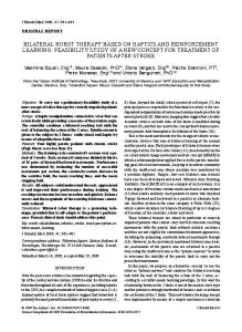
Background Agent State, 𝑠

Reward, 𝑟

Environment Policy: Decision rule 𝑠 → 𝑎

Action, 𝑎

Notation • Policy, 𝜋 𝜋 𝑎 𝑠 = Pr(𝐴𝑡 = 𝑎|𝑆𝑡 = 𝑠) • History: 𝐻 = 𝑆1 , 𝐴1 , 𝑅1 , 𝑆2 , 𝐴2 , 𝑅2 , … , 𝑆𝐿 , 𝐴𝐿 , 𝑅𝐿 • Historical data: 𝐷 = 𝐻1 , 𝐻2 , … , 𝐻𝑛 • Historical data from behavior policy, 𝜋b • Objective: 𝐽 𝜋 = 𝐄 σ𝐿𝑡=1 𝛾 𝑡 𝑅𝑡 𝜋

Agent State, 𝑠

Action, 𝑎

Reward, 𝑟

Environment

Background Observation, 𝑜

Sensors State, 𝑠

Agent Reward, 𝑟

Environment

Policy: Decision rule 𝑠 → 𝑎

Action, 𝑎

Potential Application: Digital Marketing

Potential Application: Intelligent Tutoring Systems

Potential Application: Functional Electrical Stimulation

Potential Application: Diabetes Treatment Blood Glucose (sugar)

Eat Carbohydrates

Release Insulin

Potential Application: Diabetes Treatment Blood Glucose (sugar)

Hyperglycemia

Eat Carbohydrates

Release Insulin

Potential Application: Diabetes Treatment Hyperglycemia Blood Glucose (sugar)

Hypoglycemia

Eat Carbohydrates

Release Insulin

Potential Application: Diabetes Treatment blood glucose − target blood glucose meal size injection = + 𝐶𝐹 𝐶𝑅

Potential Application: Diabetes Treatment Intelligent Diabetes Management

Motivation for Safe Reinforcement Learning • If you deploy an existing reinforcement learning algorithm to one of these problems, do you have confidence that the policy that it produces will be better than the current policy?

vs.

Learning Curves are Deceptive

• … after billions of episodes • Millions (billions?) of episodes of parameter optimization • Human intuition from past experience with these domains • Billions of episodes of experimental design

Overview • Background and motivation • Definition of “safe” • Three steps towards a safe algorithm • Off-policy policy evaluation • High-confidence off-policy policy evaluation • Safe policy improvement

• Experimental results • Conclusion

What property should a safe algorithm have? • Guaranteed to work on the first try • “I guarantee that with probability at least 1 − 𝛿, I will not change your policy to one that is worse than the current policy.” • You get to choose 𝛿 • This guarantee is not contingent on the tuning of any hyperparameters

Historical Data, 𝐷

New policy 𝜋, or No Solution Found

Probability, 1 − 𝛿 Pr 𝐽 𝜋 ≥ 𝐽 𝜋𝑏

≥1−𝛿

Limitations of the Safe RL Setting • Assumes that an initial policy is available • Often assumes that the initial policy is known • Often assumes that the initial policy is stochastic • Batch setting

Standard RL vs Safe RL Expected Return

y 𝐽(initial policy)

Episodes

Standard Safe: Pr 𝐽 𝜋 ≥ 𝐽 𝜋𝑏

≥1−𝛿

Other Definitions of “Safe”

Safe RL

Other Definitions of “Safe”

Optimization Criterion Exploration Process

Worst Case Criterion

Risk-Sensitive Criterion External Knowledge

Teacher Advice

Risk-Sensitive Criterion • Expected return:

𝐽 𝜋 = 𝐄 σ𝐿𝑡=1 𝛾 𝑡 𝑅𝑡 𝜋

Return, σ𝐿𝑡=1 𝛾 𝑡 𝑅𝑡

• Which policy is better if I am a casino? • Which policy is better if I am a doctor?

Risk-Sensitive Criterion • Idea: Change our objective to minimize a notion of risk • Penalize variance: 𝐽 𝜋 = 𝐄 σ𝐿𝑡=1 𝛾 𝑡 𝑅𝑡 𝜋 − 𝜆Var σ𝐿𝑡=1 𝛾 𝑡 𝑅𝑡 𝜋 • Maximize Value at Risk (VaR), Conditional Value at Risk (CVaR), or another robust objective

Benefits and Limitations of Changing Objectives • For some applications a risk-sensitive objective is more appropriate • Changing the objective does not address our motivation

Another notion of safety

Another Definition of Safety

Another Definition of Safety

Another Definition of Safety • Probably Approximately Correct (PAC) RL • Guarantee that with probability at least 1 − 𝛿 the policy (or 𝑞-function) will be within 𝜖 of optimal after 𝑛 episodes • Typically an equation is given for 𝑛 in terms of the number of states and actions, the horizon, 𝐿, and both 𝜖 and 𝛿 “Safe” Weak Guarantee Asymptotic convergence (expected return or risk-sensitive)

Strong Guarantee PAC

Overview • Background and motivation • Definition of “safe” • Three steps towards a safe algorithm • Off-policy policy evaluation • High-confidence off-policy policy evaluation • Safe policy improvement

• Experimental results • Conclusion

Off-Policy Policy Evaluation (OPE) • Given the historical data, 𝐷, produced by a behavior policy, 𝜋𝑏 • Given a new policy, which we call the evaluation policy, 𝜋𝑒 • Predict the performance, 𝐽 𝜋𝑒 , of the evaluation policy • Do not deploy 𝜋𝑒 since doing so could be costly or dangerous Historical Data, 𝐷 Proposed Policy, 𝜋𝑒

Estimate of 𝐽(𝜋𝑒 )

High Confidence Off-Policy Policy Evaluation (HCOPE) • Given the historical data, 𝐷, produced by the behavior policy, 𝜋𝑏 • Given a new policy, which we call the evaluation policy, 𝜋𝑒 • Given a probability, 1 − 𝛿 • Lower bound the performance, 𝐽 𝜋𝑒 , of the evaluation policy with probability 1 − 𝛿 • Do not deploy 𝜋𝑒 since doing so could be costly or dangerous Historical Data, 𝐷 Proposed Policy, 𝜋𝑒 Probability, 1 − 𝛿

1 − 𝛿 confidence lower bound on 𝐽(𝜋𝑒 )

Safe Policy Improvement (SPI) • Given the historical data, 𝐷, produced by the behavior policy, 𝜋𝑏 • Given a probability, 1 − 𝛿 • Produce a policy, 𝜋, that we predict maximizes 𝐽 𝜋 and which satisfies: Pr 𝐽 𝜋 ≥ 𝐽 𝜋𝑏 ≥ 1 − 𝛿 Historical Data, 𝐷 Probability, 1 − 𝛿

New policy 𝜋, or No Solution Found

Overview • Background and motivation • Definition of “safe” • Three steps towards a safe algorithm • Off-policy policy evaluation • High-confidence off-policy policy evaluation • Safe policy improvement

• Experimental results • Conclusion

Importance Sampling (Intuition) • Reminder:

Importance weighted return

𝑛𝑛 𝐿 𝐿 • History, 𝐻 = 𝑆1 , 𝐴1 , 𝑅1 , 𝑆2 , 𝐴2 , 𝑅2 , … , 𝑆𝐿 , 𝐴𝐿 , 𝑅𝐿 11 𝐿 𝑡 𝑖 𝑖 𝑡𝛾𝑅 𝑡𝑅 • Objective, 𝐽 𝜋e = 𝐄 σ𝑡=1 𝛾 𝑅𝑡 𝜋e 𝐽መ 𝐽መ𝜋𝜋 = = ෍ ෍ 𝑤 ෍ ෍ 𝛾 e𝑒 𝑖 𝑡𝑡

𝑛𝑛

𝑖=1 𝑖=1 𝑡=1 𝑡=1

Evaluation Policy, 𝜋e Behavior Policy, 𝜋b

Probability of history Math Slide 2/3

Importance Sampling (Derivation) • Let 𝑋 be a random variable with probability mass function (PMF) 𝑝 • 𝑋 is a history generated by the evaluation policy

• Let 𝑌 be a random variable with PMF 𝑞 and the same range as 𝑋 • 𝑌 is a history generated by the behavior policy

• Let 𝑓 be a function • 𝑓 𝑋 is the return of the history 𝑋

• We want to estimate 𝐄 𝑓(𝑋) given samples of 𝑌 • Estimate the expected return if trajectories are generated by the evaluation policy given trajectories generated by the behavior policy

• Let 𝑃 = supp 𝑝 , 𝑄 = supp(𝑞), and 𝐹 = supp(𝑓)

Importance Sampling (Derivation) • Given one sample, 𝑌, the importance sampling estimate of 𝐄𝑝 𝑓 𝑋 𝑝 𝑌 IS 𝑌 = 𝑓 𝑌 𝑞 𝑌

is:

𝑝(𝑌) 𝑝(𝑦) 𝑝(𝑥) 𝐄 𝑓(𝑌) = ෍ 𝑞(𝑦) 𝑓(𝑦) = ෍ 𝑞(𝑥) 𝑓(𝑥) 𝑞(𝑌) 𝑞(𝑦) 𝑞(𝑥) 𝑦∈𝑄

𝑥∈𝑄

= ෍ 𝑝(𝑥) 𝑓(𝑥) + ෍ 𝑝(𝑥) 𝑓(𝑥) − ෍ 𝑝 𝑥 𝑓 𝑥 𝑥∈𝑃

ത 𝑥∈𝑃∩𝑄

= ෍ 𝑝(𝑥) 𝑓(𝑥) − ෍ 𝑝 𝑥 𝑓 𝑥 𝑥∈𝑃

𝑥∈𝑃∩𝑄ത

𝑥∈𝑃∩𝑄ത

Importance Sampling (Derivation) ത • Assume 𝑃 ⊆ 𝑄 (can relax assumption to 𝑃 ⊆ 𝑄 ∪ 𝐹) 𝑝(𝑌) 𝐄 𝑓(𝑌) = ෍ 𝑝(𝑥) 𝑓(𝑥) − ෍ 𝑝 𝑥 𝑓 𝑥 𝑞(𝑌) 𝑥∈𝑃

𝑥∈𝑃∩𝑄ത

= ෍ 𝑝(𝑥) 𝑓(𝑥) 𝑥∈𝑃

=𝐄𝑓 𝑋 • Importance sampling gives an unbiased estimator of 𝐄 𝑓 𝑋

Importance Sampling (Derivation) • Assume 𝑓 𝑥 ≥ 0 for all 𝑥

𝑝(𝑌) 𝑬 𝑓(𝑌) = ෍ 𝑝(𝑥) 𝑓(𝑥) − ෍ 𝑝 𝑥 𝑓 𝑥 𝑞(𝑌) 𝑥∈𝑃

𝑥∈𝑃∩𝑄ത

≤ ෍ 𝑝(𝑥) 𝑓(𝑥) 𝑥∈𝑃

=𝐄𝑓 𝑋 • Importance sampling gives a negative-bias estimator of 𝐄 𝑓 𝑋

Importance Sampling for Reinforcement Learning • • • • • •

𝑋 ← 𝐻 produced by 𝜋𝑒 𝑌 ← 𝐻 produced by 𝜋𝑏 𝑝 ← Pr(⋅ |𝜋𝑒 ) 𝑞 ← Pr ⋅ 𝜋𝑏 𝑓 𝐻 = σ𝐿𝑡=1 𝛾 𝑡 𝑅𝑡 𝐄 𝑓 𝑋 ← 𝐽 𝜋𝑒

• IS 𝑌 =

𝑝 𝑌 𝑞 𝑌

𝑓 𝑌

• Assume either:

• Support of 𝜋𝑒 is a subset of the support of 𝜋𝑏 • Returns are non-negative

• Importance sampling estimator from one history, 𝐻 ~ 𝜋𝑏 : 𝐿 Pr 𝐻 𝜋𝑒 IS 𝐻 = ෍ 𝛾 𝑡 𝑅𝑡 Pr 𝐻 𝜋𝑏 𝑡=1

• IS(𝐻) is an unbiased estimate of 𝐽 𝜋𝑒 • Estimate from 𝐷: 𝑛 1 IS 𝐷 = ෍ IS 𝐻𝑖 𝑛 𝑖=1 𝑛

𝐿

𝑖=1

𝑡=1

1 Pr 𝐻 𝜋𝑒 = ෍ ෍ 𝛾 𝑡 𝑅𝑡 𝑛 Pr 𝐻 𝜋𝑏

Computing the Importance Weight Pr Pr

= = =

𝐻 𝜋𝑒 𝐻 𝜋𝑏 Pr 𝑆1 𝜋𝑒

Pr 𝑆1 𝜋𝑏 𝜋𝑒 𝜋𝑏

𝐴1 𝑆1 𝐴1 𝑆1

𝐴1 𝑆1 𝐴1 𝑆1

𝜋𝑒 𝐿 ς𝑡=1 𝜋

𝑏

𝜋𝑒 𝜋𝑏

Pr

Pr

𝐴2 𝑆2 𝐴2 𝑆2

𝐴𝑡 𝑆𝑡 𝐴𝑡 𝑆𝑡

𝑅1 , 𝑆2 𝑆1 , 𝐴1 𝑅1 , 𝑆2 𝑆1 , 𝐴1 … …

𝜋𝑒

𝜋𝑏

𝐴2 𝑆2 𝐴2 𝑆2

Pr(𝑅_2,𝑆_3|𝑆2 ,𝐴2 )…

Pr(𝑅_2,𝑆_3|𝑆2 ,𝐴2 )…

Importance Sampling for Reinforcement Learning 𝑛

𝐿

𝑖=1

𝑡=1

1 Pr 𝐻 𝜋𝑒 IS 𝐷 = ෍ ෍ 𝛾 𝑡 𝑅𝑡 𝑛 Pr 𝐻 𝜋𝑏 𝑛

1 = ෍ 𝑛 𝑖=1

𝐿

𝜋𝑒 𝐴𝑖𝑡 ෑ 𝜋𝑏 𝐴𝑖𝑡 𝑡=1

𝑆𝑡𝑖 𝑆𝑡𝑖

𝐿

෍ 𝛾 𝑡 𝑅𝑡 𝑡=1

Per-Decision Importance Sampling • Use importance sampling to estimate 𝐄 𝑅𝑡 |𝜋𝑒 independently for each 𝑡 𝑛

Pr 𝐻𝑡𝑖 𝜋𝑒 𝑖 1 IS𝑡 𝐷 = ෍ 𝑅𝑡 𝑖 𝑛 Pr 𝐻𝑡 |𝜋𝑏 𝑖=1 𝑛

𝑡

𝜋e 𝐴𝑗𝑖 𝑆𝑗𝑖 1 = ෍ ෑ 𝑖 𝑖 𝑛 𝜋 𝐴 𝑆 b 𝑗 𝑗 𝑖=1 𝑗=1 𝐿

𝐿

𝑛

𝑅𝑡𝑖

𝑡

𝑖 𝑖 𝜋 𝐴 1 e 𝑗 𝑆𝑗 𝑡 𝑡 PDIS 𝐷 = ෍ 𝛾 IS𝑡 𝐷 = ෍ 𝛾 ෍ ෑ 𝑖 𝑖 𝑛 𝜋 𝐴 𝑆 𝑡=1 𝑡=1 𝑖=1 𝑗=1 b 𝑗 𝑗

𝑅𝑡𝑖

Importance Sampling Range / Variance • What is the range of the importance sampling estimator? 𝑛 𝐿 𝐿 𝑖 𝑖 𝜋e 𝐴𝑡 𝑆𝑡 1 𝑡 𝑖 IS 𝐷 = ෍ ෑ ෍ 𝛾 𝑅𝑡 𝑖 𝑖 𝑛 𝜋b 𝐴𝑡 𝑆𝑡 𝑖=1

𝑡=1

𝑡=1

• Mountain car with mediocre behavior policy, 𝐿 ≈ 1000 𝜋 𝑎𝑠 • 𝑒 ∈ 0, 2.0 , σ𝐿𝑡=1 𝛾 𝑡 𝑟𝑡 ∈ 0,1 𝜋𝑏 𝑎 𝑠 • IS 𝐷 ∈ 0,21000

• The importance sampling estimator may be unbiased, but it has high variance. • Particularly when 𝜋𝑒 and 𝜋𝑏 are quite different 2 2 • MSE = Bias + Var, 𝐄 IS 𝐷 − 𝐽 𝜋𝑒 = 𝐄 IS 𝐷

− 𝐽 𝜋𝑒

2

+ Var IS(𝐷)

Importance Sampling (More Intuition) • What value does the IS estimator take in practice if 𝜋𝑒 and 𝜋𝑏 are very different? 𝑛 1 Pr 𝐻𝑖 𝜋𝑒 IS 𝐷 = ෍ Return(𝐻𝑖 ) 𝑛 Pr 𝐻𝑖 |𝜋𝑏 𝑖=1

• IS 𝐷 ≈ 0 • As 𝑛 (the number of histories in 𝐷) increases, IS 𝐷 tends towards 𝐽 𝜋𝑒 • Formally, IS 𝐷 is a strongly consistent estimator of 𝐽 𝜋𝑒 • IS 𝐷 converges almost surely to 𝐽 𝜋𝑒 as 𝑛 → ∞ • Pr lim 𝐼𝑆(𝐷) = 𝐽 𝜋𝑒 𝑛→∞

=1

An Idea • Recall that MSE = Bias2 + Var • Bias(IS) = 0 • Var(IS) = Huge • Can we make a new importance sampling estimator that has some bias, but drastically lower variance? • Perhaps make 𝐄 new estimator = 𝐽 𝜋𝑏 when there is little data • As we gather more data, have the expected value converge to 𝐽 𝜋𝑒 • The new estimator should remain strongly consistent

Weighted Importance Sampling 𝐿

𝑤𝑖 = ෑ 𝑡=1

𝜋𝑒 𝐴𝑖𝑡 𝑆𝑡𝑖 𝜋𝑏 𝐴𝑖𝑡 𝑆𝑡𝑖

𝑛

𝐿

𝑛

𝐿

𝑖=1

𝑡=1

𝑖=1

𝑡=1

𝑛

𝐿

1 𝑤𝑖 𝑖 𝑡 IS 𝐷 = ෍ 𝑤𝑖 ෍ 𝛾 𝑅𝑡 = ෍ ෍ 𝛾 𝑡 𝑅𝑡𝑖 𝑛 𝑛

WIS 𝐷 = ෍ 𝑖=1

𝑤𝑖 σ𝑛𝑗=1 𝑤𝑗

෍ 𝛾 𝑡 𝑅𝑡𝑖 𝑡=1

Weighted Importance Sampling 𝑛

WIS 𝐷 = ෍ 𝑖=1

• What if 𝑛 = 1?

𝑤𝑖

σ𝑛𝑗=1 𝑤𝑗

𝐿

෍ 𝛾 𝑡 𝑅𝑡𝑖 𝑡=1

𝐿

WIS 𝐻 = ෍ 𝛾 𝑡 𝑅𝑡𝑖 𝑡=1

• 𝐄 𝑤𝑖 = 𝐄

𝑝 𝑌 𝑞 𝑌

= σ𝑦 𝑞 𝑦

𝑝(𝑦) 𝑞(𝑦)

= σ𝑦 𝑝 𝑦 = 1

• σ𝑛𝑗=1 𝑤𝑗 → 𝑛 almost surely • WIS acts like the Monte Carlo estimator of 𝐽 𝜋𝑏 with little data and IS(𝐷) with lots of data

Off-Policy Policy Evaluation (OPE) Overview • Importance Sampling (IS) • Per-Decision Importance Sampling (PDIS) • Weighted Importance Sampling (WIS) • Others • Weighted Per-Decision Importance Sampling (WPDIS or CWPDIS) • Importance sampling with unequal support (US) • Model-based estimators (Direct Method / Indirect Method / Approximate Model) • Doubly robust importance sampling • Weighted doubly robust importance sampling • Importance Sampling (IS) + Time Series Prediction (TSP) • MAGIC (Model And Guided Importance sampling Combined)

Off-Policy Policy Evaluation (OPE) Examples

Overview • Background and motivation • Definition of “safe” • Three steps towards a safe algorithm • Off-policy policy evaluation • High-confidence off-policy policy evaluation • Safe policy improvement

• Experimental results • Conclusion

High confidence off-policy policy evaluation (HCOPE) Historical Data, 𝐷 Proposed Policy, 𝜋𝑒 Probability, 1 − 𝛿

1 − 𝛿 confidence lower bound on 𝐽(𝜋𝑒 )

Hoeffding’s Inequality • Let 𝑋1 , … , 𝑋𝑛 be 𝑛 independent identically distributed random variables such that 𝑋i ∈ [0, 𝑏] • Then with probability at least 1 − 𝛿: 𝑛 1ൗ ln 1 𝛿 𝐄 𝑋𝑖 ≥ ෍ 𝑋𝑖 − 𝑏 𝑛 2𝑛 𝑖=1

𝑛

𝐿

𝑖=1

𝑡=1

1 ෍ 𝑤𝑖 ෍ 𝛾 𝑡 𝑅𝑡𝑖 𝑛 Math Slide 3/3

Applying Hoeffding’s Inequality • Example: Mountain Car • 𝐽 𝜋𝑒 = 0.19 ∈ [0,1] • 𝑛 = 100,000 • Lower bound from Hoeffding’s inequality: −5,831,000

What went wrong? • Recall: IS 𝐷 ∈ 0,21000 • 𝑏 = 21000

1ൗ ln 1 𝛿 𝐄 𝑋𝑖 ≥ ෍ 𝑋𝑖 − 𝑏 𝑛 2𝑛 𝑛

𝑖=1

Applying Other Concentration Inequalities

See “High Confidence Off-Policy Policy Evaluation”, AAAI 2015 for how to select 𝑐𝑖

Actual

Hoeffding

Maurer & Pontil

Anderson & Massart

CUT Inequality

0.19

-5,831,000

-129,703

0.055

0.154

Approximate Confidence Intervals: 𝑡-Test 1 𝑛 σ 𝑋 𝑛 𝑖=1 𝑖

• If is normally distributed, then by Student’s 𝑡-test, with probability at least 1 − 𝛿: 𝑛 1 𝜎 𝐄 𝑋𝑖 ≥ ෍ 𝑋𝑖 − 𝑡1−𝛿,𝑛−1 𝑛 𝑛 𝑖=1

where 𝜎 is the sample standard deviation of 𝑋1 , … , 𝑋𝑛 with Bessel’s correction. 1 𝑛 • By the central limit theorem, σ𝑖=1 𝑋𝑖 is approximately normally 𝑛 distributed • If rewards non-negative then the 𝑡-test tends to be conservative.

Approximate Confidence Intervals: Bootstrap • Efron’s bootstrap, not TD’s bootstrap • Resample 𝑛 samples from 𝑋1 , … , 𝑋𝑛 with replacement to create a new data set, 𝐷1 • Repeat this process 𝛽 ≈ 2,000 times to create 𝛽 data sets, 𝐷1 , … , 𝐷𝛽

• Pretend that these 𝛽 data sets represent new independent runs • Run importance sampling (or any OPE method) on each data set: IS 𝐷1 , … , IS 𝐷𝛽 • Sort these estimates and return the 𝛿𝛽’th smallest

CI vs 𝑡-Test vs Bootstrap (non-negative rewards)

HCOPE: Mountain Car

HCOPE: Digital Marketing

HCOPE Summary • Use OPE method (e.g., importance sampling) to produce an estimate of 𝐽 𝜋𝑒 from each history • Use a concentration inequality to bound 𝐽 𝜋𝑒 given these 𝑛 estimates • Suggested method: • Weighted doubly robust + Student’s 𝑡-Test

• Suggested simple method: • Weighted per-decision importance sampling + Student’s 𝑡-Test

• Suggested method if computation is not an issue: • Weighted doubly robust + Bias-Corrected and Accelerated Bootstrap (BCa)

HCOPE Using Weighted Per-Decision Importance Sampling and Student’s 𝑡-Test

• Input: 1) 𝑛 histories, 𝐻1 , … , 𝐻𝑛 produced by a known policy, 𝜋𝑏 . 2) An evaluation policy, 𝜋𝑒 . 3) A probability, 1 − 𝛿. መ • Allocate 2-dimensional array, 𝜌 𝐿 [𝑛], and 1-dimensional arrays 𝜉 𝐿 and 𝐽[𝑛]. Initialize 𝐽መ array to zero. • For 𝑡 = 1 to 𝐿 • For 𝑖 = 1 to 𝑛 • 𝜌𝑡 𝑖 =

𝜋e ς𝑡𝑗=1 𝜋b

𝐴𝑗𝑖 𝑆𝑗𝑖

Note: More efficient implementations exist. E.g., 𝜌 𝑡 𝑖 can be computed starting from 𝜌 𝑡 − 1 𝑖

𝐴𝑗𝑖 𝑆𝑗𝑖

• 𝜉 𝑡 = σ𝑛𝑖=1 𝜌 𝑡 𝑖

• For 𝑖 = 1 to 𝑛

• For 𝑡 = 1 to 𝐿 𝜌𝑡 • 𝐽መ 𝑖 = 𝐽መ 𝑖 +

𝜉𝑡

𝑖

𝛾 𝑡 𝑅𝑡𝑖

• 𝐽 ҧ = average( 𝐽መ 1 , 𝐽መ 2 , … , 𝐽መ 𝑛 ) 2 1 σ𝑛𝑖=1 𝐽መ 𝑖 − 𝐽 ҧ 𝑛−1 𝜎 Return 𝐽 ҧ − tinv(1 − 𝛿, 𝑛 𝑛

• 𝜎= •

− 1) // See MATLAB documentation for tinv

Overview • Background and motivation • Definition of “safe” • Three steps towards a safe algorithm • Off-policy policy evaluation • High-confidence off-policy policy evaluation • Safe policy improvement

• Experimental results • Conclusion

Safe Policy Improvement (SPI) • Given the historical data, 𝐷, produced by the behavior policy, 𝜋𝑏 • Given a probability, 1 − 𝛿 • Produce a policy, 𝜋, that we predict maximizes 𝐽 𝜋 and which satisfies: Pr 𝐽 𝜋 ≥ 𝐽 𝜋𝑏 ≥ 1 − 𝛿 Historical Data, 𝐷 Probability, 1 − 𝛿

New policy 𝜋, or No Solution Found

Safe Policy Improvement • Split data, 𝐷, into two sets, 𝐷train and 𝐷test • Use batch RL algorithm on 𝐷train • Call output policy, 𝜋𝑐 , the candidate policy

• Use HCOPE algorithm and 𝐷test to lower bound 𝐽 𝜋𝑐 with probability 1 − 𝛿. Store this value in lower_bound. • If lower_bound ≥ 𝐽 𝜋𝑏 , return 𝜋𝑐 • Else, return No Solution Found, i.e., 𝜋𝑏

Safe Policy Improvement

Historical Data

Training Set (20%)

Candidate Policy, 𝜋𝑐

Testing Set (80%)

Safety Test Is 1 − 𝛿 confidence lower bound on 𝐽 𝜋𝑐 larger that 𝐽(𝜋𝑏 )?

66

Selecting the Candidate Policy Space of all policies Performance of candidate policy Best candidate policy: best performing policy that we can declare “safe”

Policy predicted to perform the best, e.g., by FQI

Tightness of performance Current policy lower bound

• Use regularization when selection candidate policy to stay “close” to the current policy.

Overview • Background and motivation • Definition of “safe” • Three steps towards a safe algorithm • Off-policy policy evaluation • High-confidence off-policy policy evaluation • Safe policy improvement

• Experimental results • Conclusion

Experimental Results: Mountain Car

Experimental Results: Mountain Car

Experimental Results: Mountain Car Natural Actor-Critic

Desired performance lower bound, −9. 5

Experimental Results: Digital Marketing

Agent State, 𝑠

Action, 𝑎

Reward, 𝑟

Environment

Expected Normalized Return

Experimental Results: Digital Marketing 0.003832

0.002715

n=10000 n=30000 n=60000 n=100000 None, CUT

None, BCa

k-Fold, CUT

k-Fold, Bca

Experimental Results: Digital Marketing

Experimental Results: Digital Marketing

Experimental Results: Diabetes Treatment

Probability Policy Worse

Probability Policy Changed

Experimental Results : Diabetes Treatment

77

Overview • Background and motivation • Definition of “safe” • Three steps towards a safe algorithm • Off-policy policy evaluation • High-confidence off-policy policy evaluation • Safe policy improvement

• Experimental results • Conclusion

Conclusion: Summary • Many definitions of “safe reinforcement learning”. • With probability at least 1 − 𝛿 the algorithm will not return a worse policy

• Three steps to making a safe reinforcement algorithm • Off-policy Policy Evaluation (OPE) • Importance sampling variants

• High Confidence Off-policy Policy Evaluation (HCOPE) • Concentration inequalities / Student’s 𝑡-Test / Bootstrap

• Safe Policy Improvement • Select candidate policy using some data and bound its performance using the rest

• Empirical Results • Safe RL is tractable!

Conclusion: Future Directions • Improvements have been by orders of magnitude. Several orders left to go. • OPE • • • • •

Can we handle long horizon problems? Can we handle non-episodic problems? What if the behavior policy is not known? What if the environment is non-stationary? How best to leverage prior knowledge like an estimate of the transition function?

• HCOPE

• Better concentration inequalities for importance sampling?

• Safe Policy Improvement

• Better techniques for selecting the candidate policy? • Automate decision of how much data to use in 𝐷train ?

Conclusion: References and Additional Reading • Importance sampling for RL (IS, PDIS, WIS, CWPDIS) • •

D. Precup, R. S. Sutton, and S. Singh. Eligibility traces for off-policy policy evaluation. In Proceedings of the 17th International Conference on Machine Learning, pages 759–766, 2000. [NOTE: WPDIS estimator has a typo] P. S. Thomas. Safe reinforcement learning. PhD Thesis, UMass Amherst, 2015.

• Doubly robust importance sampling and MAGIC for RL • •

N. Jiang and L. Li. Doubly robust off-policy value evaluation for reinforcement learning. ICML 2016 P. S. Thomas and E. Brunskill. Data-efficient off-policy policy evaluation for reinforcement learning. ICML 2016.

• Other importance sampling estimators for RL (more for bandits) • •

• • • •

P. S. Thomas and E. Brunskill. Importance Sampling with Unequal Support. AAAI 2017 P. S. Thomas., G. Theocharous, M. Ghavamzadeh, I. Durugkar, and E. Brunskill. Predictive Off-Policy Policy Evaluation for Nonstationary Decision Problems, with Applications to Digital Marketing. IAAI 2017. S. Daroudi, P. S. Thomas, and E. Brunskill. Importance Sampling for Fair Policy Selection. UAI 2017. Z. Guo, P. S. Thomas, and E. Brunskill. Using Options for Long-Horizon Off-Policy Evaluation. RLDM 2017. Y. Liu, P. S. Thomas, and E. Brunskill. Model Selection for Off-Policy Policy Evaluation. RLDM 2017. P. S. Thomas, S. Niekum, G. Theocharous, and G.D. Konidaris. Policy Evaluation Using the Omega-Return. NIPS 2015.

• HCOPE •

• • •

L. Bottou, J. Peters, J. Quinonero-Candela, D. X. Charles, D. M. Chickering, E. Portugaly, D. Ray, P. Simard, and E. Snelson. Counterfactual reasoning and learning systems: The example of computational advertising. JMLR 2013. J.P. Hanna, P. Stone, and S. Niekum. Bootstrapping with Models: Confidence Intervals for Off-Policy Evaluation. AAMAS 2017. P. S. Thomas, G. Theocharous, and M. Ghavamzadeh. High Confidence Off-Policy Evaluation. AAAI 2015. P. S. Thomas . Safe reinforcement learning. PhD Thesis, UMass Amherst, 2015.

• Safe Policy Improvement • •

P. S. Thomas, G. Theocharous, and M. Ghavamzadeh. High Confidence Policy Improvement. ICML 2015 P. S. Thomas. Safe reinforcement learning. PhD Thesis, UMass Amherst, 2015.