Toward Accurate Performance Evaluation using Hardware Counters Wiplove Mathur

Jeanine Cook

Klipsch School of Electrical and Computer Engineering New Mexico State University Box 30001, Dept. 3-O Las Cruces, NM 88003 {wmathur, jcook}@nmsu.edu

ABSTRACT On-chip performance counters are gaining popularity as an analysis and validation tool. Various drivers and interfaces have been developed to access these counters. Most contemporary processors have between two and six physical counters that can monitor an equal number of unique events simultaneously at fixed sampling periods. Through multiplexing and estimation, an even greater number of unique events can be monitored using round-robin scheduling of event sets. When program execution is sampled in multiplexed mode, the counters are interfaced to a subset of events (limited by the number of physical counters) and are incremented appropriately. At this sampling slice, the remaining events in the set do not access the counters, but the respective counts of these events are estimated. Our work addresses the error associated with the estimation of event counts during multiplexed mode. We quantify this error and propose new estimation algorithms that result in much improved accuracy.

1.

INTRODUCTION

Performance counters or Performance Monitoring Counters (PMCs) are built-in counters that are fabricated in the CPU chip. They can be programmed (by specific event-select registers) to count a specified event from a pool of events such as L1-data cache accesses, load misses, branches taken. These performance counters are the least-intrusive and an accurate technique of counting and monitoring performance [16]. Moreover, the statistics are collected in real-time and on the hardware platform that is under test, thus providing a high degree of confidence in the results. Most contemporary processors have between two and six physical counters that can monitor an equal number of unique events simultaneously. The ability of PMCs to monitor only a small number of events simultaneously limits their usage in performance analysis and validation. In contrast, simulators are widely used to gather performance data of all the desired events in a single run of the simulated architecture [18]. Behavior of different events can be correlated to different units of the microprocessor and relevant performance information can be obtained by relating different metrics to one another. With the data of various events available at the same cycle,

an accurate view of the processor state can be studied. However, when simulating only a micro-architecture (without rest of the system), the system level details (such as interfaces to buses, interrupt controllers, disks, video memory) are not taken into consideration. The behavior of a workload is affected by certain external factors (such as operating system and TLB effects [11]), which suggest that the performance data generated through simulation may not be completely accurate unless the simulator does full-system simulation (eg. Simics [3], SimOS [4]). The ability to obtain simulation-like data greatly increases the usability of PMCs for performance measurement and analysis. The paper is organized as follows: Section 2 discusses the background of interfaces to PMCs. Section 3 mentions the experimental methodology. The methodology and algorithms used to develop the estimation techniques are described in Section 4 and Section 5 discusses the results obtained by implementing the estimation algorithms. The paper concludes along with suggestions for future work in Section 6.

2. BACKGROUND 2.1 PMC Interface Several interfaces are available to access the PMCs on different microprocessor families. Some of the processor specific interfaces include Intel’s VTune software for Intel processors [5], IBM’s Performance Monitor API [14], Compaq’s Digital Continuous Profiling Infrastructure DCPI for Alpha processors [6, 7], perf-mon for UltraSPARC-I/II processors [2], and Rabbit for Intel and AMD processors [12]. Additionally, interfaces that provide portable instrumentation on multiple platforms include Performance Counter Library (PCL) [8] and Performance Application Programming Interface (PAPI) [9]. PCL and PAPI support performance counters on Alpha, MIPS, Pentium, PowerPC, and UltraSPARC processors. Moreover, PAPI explicitly supports multithreading and multiplexing. We use PAPI as our interface to access the PMCs on a Pentium-III microprocessor (refer Section 3). The normal operation of PAPI gives aggregate counts of the events that are set to be monitored by the PMCs. A Pentium-III processor has two physical counters available for monitoring desired events [1]. Therefore, a maximum of two events can be

3.1

PAPI

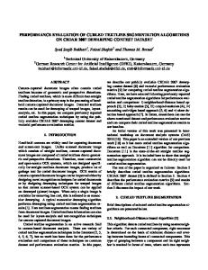
In our work, we use PAPI, version 2.3.2, to interface to the performance counters on a Pentium-III, 1GHz, dual processor machine. On this machine, we run the Red-Hat Linux 7.3 operating system, kernel version 2.4.18. The Linux kernel is patched with perfctr (version 2.4.1) which is a Linux/x86 Performance Monitoring Counters Driver [17]. PAPI uses this package to gain access to the counters on Linux/x86 platforms [10]. Figure 1: Estimation of counts of a multiplexed event in an interval. monitored simultaneously. Multiplexing is used for simultaneously counting more than two events which is described in the next section.

2.2

Multiplexed Mode

The multiplexed mode of counting is used to monitor more than one event during program execution. During each time slice, a different event is monitored as shown in Figure 1. The sequence in which the events are counted is set in an event-list. At the end of each time-slice, the current eventcount is read and stored in a file which is followed by the monitoring of the next event in the event-list(after resetting the counter). This sequence continues throughout event monitoring. For example, consider events A, B, C, and D being monitored by the counters in the multiplexed mode. Figure 1 shows a possible sequence in which the events may be monitored. An event A is physically counted only once in the entire interval. The counts corresponding to A are not known when other events (B, C, and D) are monitored. Since the aggregate count of an event corresponding to the complete interval(including the time slices when other events are monitored) is desired, an estimate value is computed by the multiplexing software. The built-in feature of multiplexing events in PAPI is used for running the counters in multiplexed mode. Since PentiumIII does not support hardware multiplexing, PAPI implements it in software. PAPI has adopted the MPX software library which is developed and implemented by May [15]. The switching of events (as described above) is triggered by using the Unix interval timer. During the initialization of the multiplexing mode, setitimer is called for setting the ITIMER PROF interval timer to a specified interval(10 milliseconds by default) and sigaction is called for setting the SIGPROF signal as a trap. When the ITIMER PROF expires, SIGPROF is sent to the process which halts the counter, stores the current count, and starts counting the next event. The counts that are not physically counted in an interval is then estimated which is discussed in Section 4.1.

3.

EXPERIMENTAL METHODOLOGY

This section describes the components of our experimental methodology. Below we describe the software we use to interface to and monitor the performance counters, the events that we monitor with this software, and the benchmarks we use in performance analysis.

The PAPI code is compiled in the DEBUG mode, and the debug data is stored in a file at the end of every time slice. The debug data is comprised of the counter values and the event ID in addition to other information. Additionally, a timer and a signal handler (similar to the one discussed in Section 2.2) is set for reading the counters at regular time slices in the non-multiplexed mode. The non-multiplexed mode of counting involves monitoring one fixed event for the complete measurement phase. As shown in Figure 2, a particular event A is monitored during every time slice. In MPX, one of the two counters is always set to read the total number of cycles(cyc) executed by the code being instrumented, whereas the second counter is used to monitor another event of interest. Therefore, we set the event-list in non-multiplexed mode such that one of the events being counted is always total number of cycles.

3.2

Benchmarks and Event Sets

We chose a subset of workloads from the SPEC CPU2000 benchmark suite [19] to use in the performance analysis of the proposed estimation techniques. These workloads and a brief description of their respective functionality are shown in Table 1. We use the reference input size in all experiments. We use a subset of events to study the accuracy of estimation techniques used in multiplexing. The Pentium-III (P6 architecture) has two performance counters that can be configured to count more than 100 events [1]. PAPI interfaces to a subset of these 100+ events. A list of these is given in Table 2. This list contains most, but not all of the events that can be monitored through PAPI. The events that we monitor and use in this work are shown in bold in Table 2. All the benchmark source codes were hand-instrumented by PAPI calls. Pseudo code for collecting the event counts in multiplexed or non-multiplexed mode is shown below:

main() { /* Benchmark variables defined*/ /* Define PAPI variables */ /* Set the timers for sampling in multiplexed / non-multiplexed mode */ /* Enable multiplex feature if counters are to be run in multiplexed mode */ /* Create the eventset */ /* Start the counters */ --- Benchmark code executes --/* Stop the counters */ return(0); }

Workload Category; Description Integer crafty Game playing; High-performance computer chess mcf Combinatorial optimization; Single-depot scheduling for mass transportation parser Word processing; Syntactic English parser twolf Computer aided design; Microchip placement and routing vpr Computer aided design; FPGA placement and routing vortex Database; Object-oriented database Floating-Point art Neural networks; Object recognition in thermal image ammp Computational chemistry; Molecular dynamics using ODEs equake Simulation; Seismic wave propagation

Table 1: Benchmarks used in Performance Analysis

Events

L1, L2, Insn and Data Caches Hits, misses, accesses, reads, writes, load/store misses, TLB misses

Category Instruction Mix total insns executed, total insn issued, FP insns executed, total branch insns executed, FP mult insns, FP div insns

(Conditional) Branch Prediction branch insns taken/not taken, branches mispredicted/predicted correctly

Table 2: Events Counted by PAPI. Events in bold type were used in study. Workload crafty mcf parser twolf vortex vpr art ammp equake

Number of intervals 5918 12578 15341 20798 3169 4777 524 27850 15312

Coefficient of Variation 0.30 0.43 0.11 0.35 0.42 0.11 0.25 0.06 0.25

Table 3: Number of multiplexed intervals collected per benchmark and Coefficient of Variation across three different execution runs. After declaring the variables of the benchmark, the PAPI library is initialized which is followed by setting the timers for the required mode. The default counting of events is in the non-multiplexed mode and hence multiplex feature is enabled if required. The eventset is created and the counters are started after which the benchmark code executes in its normal sequence. The counters are read at regular time slices and are stopped just before the completion of the benchmark.

4.

2. The non-multiplexed data vector consists of six counts for each equivalent multiplexed interval. The sum of these six counts is the non-multiplexed (count nmi ) event count. 3. The multiplexed event count (count mi ) is estimated for every interval using an algorithm described in the following sections. 4. The estimation error, |count mi − count nmi |, for every interval is calculated.

METHODOLOGY AND ALGORITHMS

The workloads are instrumented with the multiplexed and non-multiplexed code (as discussed in Section 3.2) for monitoring six different events (Table 2). We execute an individual workload in each mode three times. We do this to reduce the error due to variability of data collection in different executions of the same workload. Our aim is to obtain minimum absolute error between the multiplexed and the nonmultiplexed counts in every interval. The non-multiplexed counts reflect the actual/accurate count of an event since it is monitored continuously throughout the execution of the workload which is not the case in multiplexed counts (refer Section 2.2). The steps followed to calculate the statistics are as follows: 1. Workloads are executed as mentioned above.

Table 3 shows the number of multiplexed intervals that occur in the full execution of each workload, where an interval is defined to contain a time slice during which one of the multiplexed events is counted and the remaining event counts are estimated. Coefficient of Variation is calculated across the 3 execution runs of the benchmark in multiplexed mode (refer Section 4). Figure 2 shows the format of the data obtained by reading the counters(in non-multiplexed and multiplexed modes) at regular time slices. cyci(k) is the total number of cycles elapsed, starting from the instant the code is being instrumented. i is the ‘interval’ in which all the multiplexed events are being physically monitored once by the PMC and k is the ‘time slice’ (finest granularity) for which a counter is accumulating event occurrences (after resetting the counter

slopei =

rate mi − rate m(i−1) cyci(n) − cyci−1(n)

(4)

where n = the number of events being multiplexed. In our study, n=6. k = the time slice during which the event-count is sampled rate mi and rate nmi(k) = rate of occurrence of an event in multiplexed and non-multiplexed mode respectively Figure 2: Data format of non-multiplexed and multiplexed counters at regular time slices.

count mi(n) = the number of times an event has occurred in the ith interval and in time slice between cyci(n−1) and cyci(n) count nmi(k) = the number of times an event has occurred in the kth time slice of ith interval (that is the period between cyci(k−1) and cyci(k) ) slopei = slope of rate between i − 1th and ith intervals We discuss the estimation algorithms in the following section.

4.1

Base Algorithm

The estimation algorithm(henceforth called Base Algorithm) used in PAPI is developed and implemented by May [15]. It is used to estimate the counts of the multiplexed event in each interval.

Figure 3: Conversion of event counts to respective rates in multiplexed mode. at the end of time slice k-1 ). Therefore, if n events are being multiplexed, then k can take values from 0 to n. For simplicity, we assume cyci(n) to be equivalent to cyci+1(0) . Figure 3 shows the rate plot of all the events measured in the multiplexed mode. Some important variables (at the ith interval, kth time-slice) that are used in this paper are listed below.

rate mi =

rate nmi(k) =

count mi(n) cyci(n) − cyci(n−1)

count nmi(k) ; cyci(k) − cyci(k−1)

count nmi =

n X k=1

0≤k≤n

count nmi(k)

(1)

(2)

(3)

Figure 4: Event-count calculation of a multiplexed event using base algorithm Consider the case as shown in Figures 2 and 3. We discuss the base algorithm that is used to estimate the count of event A in the ith interval. Event A is monitored in the time slice k =4 (from total cycles cyci(3) to cyci(4) ). If count mi(4) is the number of occurrences of event A in this time slice, then the rate of event A can be calculated using Eqn. 1 as:

rate mi =

count mi(4) cyci(4) − cyci(3)

(5)

Figure 4 shows the plot of Rate vs. Total Cycles for event A alone. The rate of event A, rate mi and rate mi−1 , corresponding to intervals i and i-1 respectively, can be calculated using eqn. 5. In the base algorithm, rate mi is assumed to be constant for the entire ith interval and the count of event A is estimated by the following equation:

count mi ≈ rate mi · (cyci(n) − cyci−1(n) )

(6)

Recall that rate mi is calculated using the data corresponding to the period between i(n-1) and i(n) (that is 1 time slice), whereas the count between i-1(n) and i(n) (that is 1 interval) is being estimated.

4.2

Trapezoid-area Method (TAM)

Figure 6: Event-count calculation of a multiplexed event using Divided-interval Rectangulararea method or DIRA divided or split into j equal parts (see Figure 6). The rate at the kth division is calculated by using linear interpolation as follows: rate mi(k) = slopei · (cyci(k) − cyci−1(n) ) + rate mi−1 (8) where slopei is given by Eqn. 4. 2. The area corresponding to kth division is calculated by assuming the rate to remain constant between cycles cyci(k−1) and cyci(k) . Thus, the area under rectangle PQRS in Figure 6 is given by the formula:

Figure 5: Event-count calculation of a multiplexed event using Trapezoid-area method Figure 5 shows the plot of Rate vs. Total Cycles for an event A which is being multiplexed. The rate of event A, rate mi and rate mi−1 , corresponding to intervals i and i-1 respectively, is calculated using eqn. 5. In the trapezoid-area method, the rate of occurrence of event A is assumed to be linearly changing within an interval. Thus, the estimated count of the multiplexed event A in the ith interval is given by the area under the trapezoid PQRS (refer Figure 5). Mathematically,

count mi(k) ≈ rate mi(k) · (cyci(k) − cyci(k−1) )

(9)

where value of rate mi(k) is obtained from Eqn. 8. 3. Repeat steps 1 and 2 for 1 ≤ k ≤ j 4. The estimated count of the multiplexed event A in the ith interval is given by:

count mi =

j X

count mi(k)

(10)

k=1

count mi ≈ 0.5 · (rate mi + rate mi−1 ) · (cyci(n) − cyci−1(n) ) (7)

4.3

Divided-interval Rectangular Area method (DIRA)

We describe a simple algorithm called Divided-interval Rectangular area method (DIRA) for estimating the count of an event, A. Figure 6 shows the plot of Rate vs. Total Cycles for an event A which is being multiplexed. The rate of event A, rate mi and rate mi−1 , corresponding to intervals i and i-1 respectively, is calculated using eqn. 5. The algorithm is explained in the following steps: 1. The ith interval (where the count is being estimated) is

In our case, j =n(=6).

4.4

Positional Mean Error (PME)

The Positional Mean Error (PME) algorithm is a 2-phase algorithm. Phase-1 involves calculating the rate corrections or the positional mean errors and Phase-2 consists of using the PMEs to correct the multiplexed rates and estimate the event count. The following steps comprise Phase-1: 1. The rate of event A in multiplexed mode at the kth position, (rate mi(k) ), is calculated by using linear interpolation:

4. Estimated count in the ith interval is then given by: count mi =

n X

count mi(k)

(16)

k=1

4.5

Multiple Linear Regression Model (MLR)

The Multiple Linear Regression model (MLR) allows prediction of a response variable as a function of predictor variables using a linear model [13]. In vector notation, it is given by:

y = Xb + e

(17)

where Figure 7: Event-count calculation of a multiplexed event using Positional Mean Error method

rate mi(k) = slopei · (cyci(k) − cyci−1(n) ) + rate mi−1 (11)

y = a column vector of the non-multiplexed counts when aggregated in respective multiplexed intervals. X = matrix where each column element is the dividedinterval trapezoidal area as shown in Figure 8 and the data in a specific row corresponds to a particular interval. b = Predictor parameters

where slopei is given by Eqn. 4. 2. The difference between the rate of event A in nonmultiplexed mode, rate nmi(k) and the rate that is calculated in Step 1 above is given by: ek = rate nmi(k) − rate mi(k)

(12)

This is shown in Figure 7 and rate nmi (k) is given by Eqn. 2. This difference is the positional error (for position k ) in the ith interval and is calculated for 1 ≤ k ≤ n and ∀i (n=6 in our case). 3. The PME is then given by: pmek =

1 itotal

·

X

ek

(13)

∀i

where pmek is the Positional Mean Error for the kth position and itotal is the total number of intervals. Phase-1 produces n PMEs that are used in Phase 2 for estimating the event counts. Phase 2 includes the following steps:

Figure 8: Event-count calculation of a multiplexed event using MLR

Hence, the multiplexed sub-interval areas are represented as a linear model of the actual count (the non-multiplexed count). The predictor parameter estimation is given by:

1. Same as Step 1 of Phase-1 2. Calculate the corrected rate at kth position ∀k. c rate mi(k) = rate mi (k) + pmek

b = (X T X)−1 (X T y)

(18)

(14)

3. Assuming linear rate between corrected positional rates, the count in the kth slice-division is now estimated using the trapezoid area method discussed in Section 4.2 count mi(k) ≈ 0.5 · (c rate mi(k) + c rate mi(k−1) ) · (cyci(k) − cyci(k−1) ) (15)

The estimated parameter is then used to scale the trapezoid area in an interval and the sum of the scaled area is estimated as the multiplexed count of that interval. Mathematically,

scaled xk = b[k] · xk

(19)

j

count mi =

X

scaled xk

(20)

k=1

For our study, the sample size = 0.5 of the population size.

5.

RESULTS

The error in the base algorithm is computed by comparing the estimated multiplexed counts to the non-multiplexed counts of the same event. We distributed the errors in 5 groups: less than 5%, 5-10%, 10-15% and above 50%. Table 4 lists the acronyms used for the six events being multiplexed and figures 9 and 11 show the histogram for integer and floating point workloads respectively. The histograms indicate a very high percentage of interval counts in multiplexed mode being inaccurately estimated. This behavior is observed for all the integer (with the exception of twolf ) and floating point workloads. For instance, while estimating the count for store misses (stm) in mcf (Figure 9(b)), as much as 51% of the intervals were estimated with above 50% error and 42% of the intervals were estimated with 15-50% error. Almost all the events in every workload has at least 50% of the intervals being estimated with more than 5% error. A similar behavior is observed in the floating point workloads with as much as 93% intervals being estimated with greater than 50% error for the store misses in quake (Figure 11(c)). This shows that the estimation accuracy of the base algorithm is very low. We show the results of applying the algorithms described in section 4.1 through 4.5 in Figures 10 and 12. They describe the accuracy of each algorithm for each event in terms of error. The error in the algorithm is computed by comparing the estimated multiplexed counts to the nonmultiplexed counts of the same event. The total absolute P error ( ∀k |count mk − count nmk |) is computed for all the algorithms and compared with the base. Each data point is normalized to the error computed for the base algorithm. Values less than 1 indicates lesser error in the estimation of multiplexed counts. Lower the normalized values, better is the algorithm. For all the benchmarks, the proposed estimation algorithm result in decreased error compared to the base algorithm for each event. For the benchmark crafty, the reduction of error varies between 10-40% over the set of events as shown in Figure 10(a). For data cache misses (dcm) and load misses (ldm), the error reduction realized by PME and MLR is around 40%. TAM and DIRA in general resulted in smaller error reductions. For crafty, this is around 10% for both TAM and DIRA. Similar improvements are observed for the floating point benchmarks shown in Figure 12. The error reduction varies between 7-40% for all the floating point workloads across the six events. MLR proved to be the best algorithm for quake which produced an estimation error reduction of almost 40% for the store misses (stm).

6.

CONCLUSIONS AND FUTURE WORK

The algorithms discussed in this paper reduce the estimation error for all the multiplexed events for all the workloads. Improvement of up to 40% is achieved by PME and MLR

Event L1 Data Cache Misses L1 Data Cache Access Instructions Committed L1 Load Misses L1 Store Misses Conditional Branches taken

Acronym dcm dca ins ldm stm brtkn

Table 4: Acronym table for the multiplexed events monitored algorithms and up to 30% for TAM and DIRA. Utilizing any of these techniques will greatly reduce the estimation errors of the multiplexed counts. PME and MLR require a pre-calculated library of correction parameters (corresponding to the event-workload pair) for their implementation whereas TAM and DIRA are more generic and independent of any event or workload. Since the interval size is defined by time (10 miiliseconds in our case), the event counts cannot be collected at a specified cycle. Therefore, it is difficult to collect cycle-synchronized performance metrics that can provide a complete snapshot of program behavior. We plan to address this in the future by implementing an algorithm that we have developed into the techniques discussed in this paper.

100 80

80

70

70

60 50 40 30

60 50 40 30

20

20

10

10

0

dcm

dca

ins

Events

ldm

stm

< 5% 5−15% 15−50% > 50%

90

% of multiplexed intervals

% of multiplexed intervals

100

< 5% 5−15% 15−50% > 50%

90

0

brtkn

dcm

dca

(a) crafty 100

70

% of multiplexed intervals

% of multiplexed intervals

80

70 60 50 40 30

30 10

ldm

stm

< 5% 5−15% 15−50% > 50%

40 20

Events

0

brtkn

dcm

dca

(c) parser

Events

ldm

stm

brtkn

vpr

100

< 5% 5−15% 15−50% > 50%

90

< 5% 5−15% 15−50% > 50%

90

80

80

70 % of multiplexed interval

% of multiplexed intervals

ins

(d) twolf

100

60 50 40 30 20

70 60 50 40 30 20

10 0

brtkn

50

10 ins

stm

60

20

dca

ldm

90

80

dcm

Events

100

< 5% 5−15% 15−50% > 50%

90

0

ins

(b) mcf

10 dcm

dca

ins

Events

ldm

(e) vortex

stm

brtkn

0

dcm

dca

ins

Events

ldm

stm

brtkn

(f) vpr

Figure 9: Histogram plot showing inaccuracy distribution of errors in estimating multiplexed event counts (Integer benchmarks)

Base PME MLR TAM DIRA

1 0.8

0.8

0.6

0.6

0.4

0.4

0.2

0.2

0

dcm

dca

ins

Events

ldm

stm

0

brtkn

Base PME MLR TAM DIRA

1

dcm

dca

(a) crafty Base PME MLR TAM DIRA

1

0.8

0.6

0.6

0.4

0.4

0.2

0.2

dcm

dca

ins

Events

ldm

stm

0

brtkn

Base PME MLR TAM DIRA

0.8

0.6

0.6

0.4

0.4

0.2

0.2

ins

Events

ldm

(e) vortex

brtkn

dcm

dca

ins

Events

ldm

stm

brtkn

stm

brtkn

Base PME MLR TAM DIRA

1

0.8

dca

stm

(d) twolf

1

dcm

ldm

Base PME MLR TAM DIRA

(c) parser

0

Events

1

0.8

0

ins

(b) mcf

0

dcm

dca

ins

Events

ldm

stm

brtkn

(f) vpr

Figure 10: Total absolute error of the estimated multiplexed counts (normalized to the base algorithm): Integer benchmarks

Base PME MLR TAM DIRA

1 100

< 5% 5−15% 15−50% > 50%

90

0.8

% of multiplexed intervals

80

0.6

70 60

0.4

50 40 30

0.2

20 10 0

0 dcm

dca

ins

Events

ldm

stm

dcm

dca

brtkn

ins

Events

ldm

stm

brtkn

(a) art

(a) art

Base PME MLR TAM DIRA

1.356

100

< 5% 5−15% 15−50% > 50%

90

% of multiplexed intervals

80

1 0.8

70 60

0.6

50 40

0.4

30 20

0.2

10 0

dcm

dca

ins

Events

ldm

stm

brtkn

0

(b) ammp

dcm

dca

ins

Events

ldm

stm

brtkn

(b) ammp fquake

100

< 5% 5−15% 15−50% > 50%

90

Base PME MLR TAM DIRA

1

% of multiplexed intervals

80 70

0.8

60 50

0.6

40 30

0.4

20 10 0

dcm

dca

ins

Events

ldm

stm

brtkn

(c) quake Figure 11: Histogram plot showing inaccuracy distribution of errors in estimating multiplexed event counts (Floating point benchmarks)

0.2 0

dcm

dca

ins

Events

ldm

stm

brtkn

(c) quake Figure 12: Total absolute error of the estimated multiplexed counts (normalized to the base algorithm): Floating point benchmarks

7.

REFERENCES

[1] Intel architecture software developer’s manual, volume 3: System programming guide. Intel document number 243192, http://developer.intel.com/. [2] Perf-monitor for UltraSPARC. http://www.sics.se/ mch/perf-monitor/. [3] SIMICS, www.simics.com. [4] The SimOS complete system simulator, http://simos.stanford.edu/. [5] Vtune profiling software, http://www.intel.com/software/products/vtune/. [6] DIGITAL continuous profiling infrastructure project. http://www.research.digital.com/SRC/dcpi/, Oct 1997. [7] J. Anderson, L. Berc, J. Dean, S. Ghemawat, M. Henzinger, S. Leung, D. Sites, M. Vandevoorde, C. Waldspurger, and W. Weihl. Continuous profiling: Where have all the cycles gone, 1997. [8] R Berrendorf, Heinz Ziegler, and Bernd Molar. PCL the performance counter library: A common interface to access hardware performance counters on microprocessors. Research Centre Juelich GmbH, http://www.fzjuelich.de/zam/PCL/Version 2.1, February 2002. [9] S. Browne, J. Dongarra, N. Garner, G. Ho, and P. Mucci. A portable programming interface for performance evaluation on modern processors. The International Journal of High Performance Computing Applications, 14(3):189–204, Fall 2000. [10] J. Dongarra, K. London, S. Moore, P. Mucci, and D. Terpstra. Using PAPI for hardware performance monitoring on linux systems. In Conference on Linux Clusters: The HPC Revolution, June 25-27 2001. [11] Jeff Gibson, Robert Kunz, David Ofelt, and Mark Heinrich. FLASH vs. (simulated) FLASH: Closing the simulation loop. In Architectural Support for Programming Languages and Operating Systems, pages 49–58, 2000. [12] Don Heller. Rabbit: A performance counters library for Intel/AMD processors and linux. http://www.scl.ameslab.gov/projects/rabbit/. [13] Raj Jain. The Art of Computer Systems Performance Analysis: Techniques for Experimental Design, Measurement, Simulation and Modeling. John Wiley & Sons, Inc., 1991. [14] F.E. Levine and C.P. Roth, editors. A programmer’s view of performance monitoring in the PowerPC microprocessor., number 41(3). IBM Journal of Research and Development, May 1997. [15] John M. May. MPX: Software for multiplexing hardware performance counters in multithreaded programs. In Parallel and Distributed Processing Symposium., Proceedings 15th International, pages 8 –, April 2001.

[16] Anand. K. Ojha. Techniques in least-intrusive computer system performance monitoring. In SoutheastCon 2001. Proceedings. IEEE, pages 150–154, 2001. [17] Mikael Pettersson. Linux x86 performance-monitoring counters driver. http://www.csd.uu.se/ mikpe/linux/perfctr/. [18] Kevin Skadron, Margaret Martonosi, David I. August, Mark D. Hill, David J. Lilja, and Vijay S. Pai. Challenges in computer architecture evaluation. IEEE Computer, August 2003. [19] Standard Performance Evaluation Corporation (SPEC). http://www.spec.org.