1
Turbo receivers for Space-Time BICM Bogdan Cristea
Abstract In this paper several algorithms suitable for turbo reception in Space-Time (ST) Bit-Interleaved Coded-Modulation (BICM) systems are discussed. First, an equivalent channel including both the ST code and the Multiple-Input Multiple-Output (MIMO) channel is deduced. Based on the equivalent channel model, a general structure of the turbo receiver is proposed. Different choices for the algorithms to use in the Soft-Input Soft-Output (SISO) demapper are discussed and compared with respect to their complexities and performances. It is also shown that all previously presented algorithms can be seen as particular cases of the Probabilistic Data Association (PDA) algorithm. The application of the PDA algorithm allows for faster convergence and lower complexity of the turbo receiver.
Index Terms turbo receivers, space-time block codes, bit-interleaved coded-modulation
I. I NTRODUCTION Increased capacity and reliable communication over fading channels are the main concerns of modern wireless communication systems. A possible answer to these concerns is represented by MIMO systems which, together with Orthogonal Frequency Division Multiplex (OFDM) modulation, can ensure both capacity and performance improvement over fading channels needed for future wireless systems. ST processing techniques have been an intensively research subject in the past years [1], [2], [3]. ST trellis codes [1] and ST block codes [2] are among the best known ST processing techniques. While the ST trellis codes have the disandvantage of exponentially increasing complexity with the constraint length of the code and the transmission rate [1], ST block codes offer a good tradeoff between performances and complexity [2], [3]. In order to attain the channel capacity promised by the Shannon formula, turbo processing techniques for MIMO systems were developed [4]. Several turbo reception techniques were August 5, 2009
DRAFT
2
proposed for ST block codes [5], [6], [7], [8]. All these techniques use at the transmitter side a Forward Error Correcting (FEC) code whose coded bits are interleaved and mapped into symbols from a given contellation. Space-time processing follows and then the processed symbols are send into a MIMO channel. The turbo receiver is based on two SISO blocks separated by interleavers. The two SISO blocks exchange extrinsic informations along several iterations, after which the decision is made in order to recover the informational bits. Our paper aims to extend previous work related to turbo receivers for MIMO systems and to provide new results. Using a general framework, which includes all existing ST block codes, we compare several turbo receivers. The MIMO system model we use is based on BICM system model. The reason behind our choice is the fact that existing BICM systems can be easily extended to a space-time version by adding a ST code after the modulator. However, the results provided here can be easily extended for other MIMO systems using other transmitter structures. The rest of the paper is organized as follows. In section II the system model is presented and an equivalent channel model is deduced. The equivalent channel includes both the ST code and the MIMO channel. Using the equivalent channel model, in section III the general structure of the turbo receiver is presented. Several algorithms, suitable for turbo reception in MIMO systems, are described. Section IV compares these algorithms with respect to their complexities and performances. Finally, some conclusions are given in section V. Notations: Lowercase bold letters are used for vectors and uppercase bold letters for matrices. Given a complex number a ∈ C, Re[a] and Im[a] denote its real and imaginary part respectively.
a∗ stands for the complex conjugate of the complex number a. A complex matrix A with M
lines and N columns is denoted as A ∈ CM ×N . AT and AH denote the transpose and the Hermitian transpose respectively of the complex matrix A. A(i, :) is the i-th line of the matrix P A. The trace of a square matrix A = {aij } ∈ CN ×N is tr[A] = N i=1 aii . II. S YSTEM
MODEL
We consider a transmission system based on BICM, where a ST block code is applied after the Quadrature Amplitude Modulation (QAM) modulator (Fig. 1). Such a scheme was nicknamed ST BICM [5]. The motivation behind the use of ST codes in BICM systems is the capacity increase and performance improvement in fading channels due to emission and reception diversity. [Fig. 1 about here.] August 5, 2009
DRAFT
3
In our model, the FEC code is a nonrecursive and nonsystematic convolutional code of coding rate ρ. Coded bits are interleaved by a random interleaver, π(n). Succesive frames of m bits are then transformed into QAM symbols using Gray mapping. The mapping choice can affect considerably system performances when turbo receivers are used [9], but here we have chosen to fix the mapping in order to compare different turbo receivers for ST BICM systems. The symbols obtained at the modulator output, sq ∈ C, are normalized in order to have an unitary mean symbol energy: E[sq ] = 1. Thus, the mean emitted energy is independent of the modulation order. Further, each symbol is multiplied by the constant
√1 , M
where M is the number
of emission antennas, so that the energy received by one antenna is independent of the number of emission antennas. Frames of Q symbols are then transformed by the ST block code into matrices S with M lines and Q columns. In a symbol duration, one column of the matrix S is emitted over M antennas, so that the entire matrix is transmitted during T symbol durations. The coding rate of the ST code can be defined as [2]: R=
Q T
(1)
From (1), the spectral efficiency of the system, η, is: η = ρmR [bits/symbol duration]
(2)
Any ST block code, defined by the matrix S, can be represented as a linear combination of Q symbols sq [2]: Q−1
S=
X
(Aq Re[sq ] + Bq Im[sq ])
(3)
q=0
where Aq , Bq ∈ CM ×T are the generating matrices of the ST block code. For mathematical simplicity we have considered symbols, sq , only from one frame of Q symbols. The codes defined by (3) are also known as linear-dispersion codes and were optimized in [2] to maximize the mutual information. In order to have the energy contained by the matrix S independent of the ST code, the matrix S must satisfy the constraint: E[tr[SSH ]] = T M
(4)
This constraint can be easily satisfied using normalized generating matrices, Aq and Bq .
August 5, 2009
DRAFT
4
Examples of ST codes descibed by (3) are the Vertical Bell Laboratories Layered Space-Time (V-BLAST) code (Q = M and T = 1) [10] h iT S = s0 s1 · · · sQ−1 the Alamouti code (Q = 2, M = 2 and T = 2) [11] s0 −s∗1 S= s1 s∗0
and the golden code (Q = 2, M = 2 and T = 2) [3] α(s + s θ) α(s + s θ) 1 0 1 2 3 S= √ ¯ α(s ¯ 5 γ α(s ¯ 2 + s3 θ) ¯ 0 + s1 θ) where θ =
√ 1+ 5 , 2
(5)
(6)
(7)
¯ and γ = . θ¯ = 1 − θ, α = 1 + (1 − θ), α ¯ = 1 + (1 − θ)
Note that the V-BLAST code (5) has a maximum coding rate R = Q (high spectral efficiency), but no emission diversity, since different symbols are emitted on each antenna. The orthogonal code of Alamouti (6) has a coding rate of R = 1, but maximum emission diversity, since, the two symbols, s1 and s2 , are emitted alternatively on each of the two antennas. A compromise sollution, with respect to previously presented ST block codes, is represented by the golden code (7), which has maximum coding rate, R = 2, and maximum emission diversity. The golden code is among the best known ST block codes with respect to performances and spectral efficiency [3]. The propagation channel is supposed flat-fading and constant during T symbol durations. More complex channel models, like the multipath channels, can be reduced to the flat-fading model by using the OFDM and the cyclic prefix. The received signal, X ∈ CN ×T , can be written as: X = HS + η
(8)
where H ∈ CN ×M is the channel matrix and can be different from one block of code S to the next one. In our model, the elements of the channel matrix, H, follow a Rayleigh distribution with variance 1/2 on each dimension. N is the number of reception antennas and η ∈ CN ×T is the Additive White Gaussian Noise (AWGN) with σ 2 the noise variance on each dimension.
The MIMO channel represented by (8) can be written as an equivalent real channel, including the influence of the ST code [2]: xeq = Heq seq + η eq August 5, 2009
(9) DRAFT
5
where xeq ∈ R2N T ×1 is the equivalent received signal: h iT xeq = Re[X(0, :)] Im[X(0, :)] Re[X(1, :)] · · · Im[X(N − 1, :)]
(10)
and η eq ∈ R2N T ×1 is the equivalent Gaussian noise: h iT η eq = Re[η(0, :)] Im[η(0, :)] Re[η(1, :)] · · · Im[η(N − 1, :)]
(13)
Heq ∈ R2N T ×2Q is the equivalent channel matrix: A h Beq,0 h0 · · · Aeq,Q−1 h0 Beq,Q−1h0 eq,0 0 .. .. . .. . . . Heq = (11) . . . . . Aeq,0 hN −1 Beq,0 hN −1 · · · Aeq,Q−1 hN −1 Beq,Q−1hN −1 T T h iT Re[Ai] Im[Ai ] − Im[Bi ] Re[Bi] Aeq,i = , Beq,i = , hi = Re[H(i, :)] Im[H(i, :)] , − Im[Ai ] Re[Ai ] − Re[Bi ] − Im[Bi ] seq ∈ R2Q×1 is the equivalent vector of emitted symbols: iT h seq = Re[s0 ] Im[s0 ] Re[s1 ] · · · Im[sQ−1 ] (12)
The equivalent channel (9) allows to pass from a complex MIMO channel (8), with complex
matrices as input and output signals, to a real MIMO channel (9) with real vectors at its input and output. This model can also take into account an arbitrary ST block code. Thus the implementation of generic turbo receivers for MIMO systems, using any ST block code, is simplified. Different choices for turbo receivers will be discussed in the following. III. T URBO
RECEIVERS
The general structure of the turbo receiver is described in Fig. 2. [Fig. 2 about here.] The SISO demapper outputs extrinsic information of coded bits, L(cn ; O), based on the received signal, X (8), and the a priori information of coded bits L(cn ; I). The extrinsic information L(cn ; O) is transferred, after inverse interleaving, as intrinsic information to the SISO Decoder (DEC). This module decodes the FEC (convolutional code) and outputs an extrinsic information of coded bits, which becomes, after interleaving, a priori information at the SISO demapper
August 5, 2009
DRAFT
6
input L(cn ; I). At the last iteration, the Logarithm of Likelihood Ratio (LLR) of informational bits from the SISO DEC, Λ(bk ), is used in order to recover the informational bits. The SISO DEC utilizes the Maximum A Posteriori (MAP) algorithm [12] in order to compute the soft informations. In the SISO demapper, the MIMO channel and the ST code are considered as an equivalent channel and decoded using equation (9). In order to compute the extrinsic information, L(cn ; O), several algorithms can be used. These algorithms are the main scope of this paper and will be described in the following. A. MAP algorithm A first choice for the SISO demapper is represented by the MAP algorithm [5], adapted to take into account the equivalent channel (9) and the QAM modulator (Fig. 1). The starting point is represented by the LLR of coded bits, Λ(cn ): P (cn = 1/xeq ) P (cn = 0/xeq )
def
Λ(cn ) = ln
(14)
Using the Bayes’ rule in (14) one can obtain the extrinsic information of coded bits, L(cn ; O), as: L(cn ; O) = Λ(cn ) − L(cn ; I)
(15)
where L(cn ; I) is the a priori information of coded bits: def
L(cn ; I) = ln In order to obtain Λ(cn ), (14) is rewritten as: P
P (cn = 1) P (cn = 0)
seq ∈S1
Λ(cn ) = ln P
seq ∈S0
(16)
P (seq /xeq )
(17)
P (seq /xeq )
where S1 is the set of vectors seq (12) having on the n-th position the bit cn = 1, n ∈ {0, 1, . . . , mQ − 1}. With the Bayes’ rule in (17), Λ(cn ) can be obtained as: P s ∈S p(xeq /seq )P (seq ) Λ(cn ) = ln P eq 1 seq ∈S0 p(xeq /seq )P (seq )
(18)
where p(xeq /seq ) is the probability density function of the equivalent received vector xeq , knowing the equivalent emitted vector seq : p(xeq /seq ) =
August 5, 2009
1 (2π)N T σ 2N T
(xeq − Heq seq )T (xeq − Heq seq ) exp − 2σ 2
!
(19)
DRAFT
7
and P (seq ) is the a priori probability of the equivalent emitted vector. If the coded bits, cn , n ∈ {0, 1, . . . , mQ − 1}, corresponding to the equivalent emitted vector, are independent, then P (seq ) can be written as: P (seq ) = ΠmQ−1 i=0 P (ci )
(20)
Knowing that (16) P (ci) =
exp(ci L(ci ; I)) 1 + exp(L(ci ; I))
(21)
and using the approximation ln(exp(a) + exp(b)) ≈ max(a, b)
(22)
one can obtain a simplified expression for Λ(cn ) (17): Λ(cn ) = max
seq ∈S1
max
seq ∈S0
−
T
(xeq − Heq seq ) (xeq − Heq seq ) + 2σ 2
mQ−1
X i=0
!
ci L(ci ; I) −
mQ−1 X (xeq − Heq seq )T (xeq − Heq seq ) − ci L(ci ; I) + 2σ 2 i=0
!
(23)
The computation of the extrinsic information (15) using the MAP algorithm has a complexity exponential with the product between the number of bits per symbol, m, and the number of symbols per block, Q: � O mQ2mQ (2(2Q)(2NT ) + 2NT + mQ + 1)
(24)
The complexity of the MAP algorithm was computed by considering combinations of 2mQ−1 bits in (23) for every of the mQ bits in a block of ST code. The number of multiplications needed in (23) was also taken into account. When computing the complexity of the MAP algorithm, we have not considered the complexity implied by the computation of the equivalent channel, (10) and (11), since this one is the same for all considered algorithms and our goal is to compare these algorihms with respect to their performances and complexity. Thus, the number of emission antennas, M, is not included in the formula for the complexity of the MAP algorithm. Following (24), the implementation of the MAP algorithms is too complex in most cases. The presentation of the MAP algorithm is useful since this is the optimal algorithm to use in the SISO demapper and allows to compare the performances of lower complexity algorithms. These algorithms will be described in the following subsections. August 5, 2009
DRAFT
8
B. Gaussian Approximation The algorithm based on the Gaussian Approximation (GA) utilises the hypothesis that the Co-Antenna Interference (CAI) can be seen as a random variable [13], [8]. If the number of interfering antennas is large enough, then, using the central limit theorem, one can consider that the CAI is a random Gaussian variable. In the case of the equivalent channel (9), the current equivalent symbol, seq,q , (the real or the imaginary part of the real emitted symbol sq ) can be separated from the interference of other symbols (antennas): xeq = Heq (:, q)seq,q + ζ q
(25)
where ζ q ∈ R2N T ×1 represents the interference of other symbols and the AWGN 2Q−1
ζq =
X
Heq (:, i)seq,i + η eq
(26)
i=0 i6=q
and Heq (:, i) is the i-th column of the matrix Heq (11). Note that in our equivalent channel model (9) the number of interfering antennas is 2Q − 1 (26). According to the above hypothesis, ζ q is a vector of random Gaussian variables: ζ q ∼ � N E[ζ q ], Cov[ζ q ] , where the mathematical expectation, E[ζ q ], and the covariance matrix, Cov[ζ q ],
of the vector ζ q are obtained from the a priori probability P (seq,i ): 2Q−1
E[ζ q ] =
X
Heq (:, i) E[seq,i ]
(27)
i=0 i6=q
= E[xeq ] − Heq (:, i) E[seq,i] where
(28)
2Q−1
E[xeq ] =
X
Heq (:, i) E[seq,i]
(29)
i=0
and
� � � � � � Cov[ζ q ] = E ζ q ζ Tq − E ζ q E ζ Tq
(30)
2Q−1
=
X
Heq (:, i)HTeq (:, i) Var[seq,i] + σ 2 I2N T
(31)
i=0 i6=q
= Cov[xeq ] − Heq (:, q)HTeq (:, q) Var[seq,q ] August 5, 2009
(32) DRAFT
9
where
2Q−1
Cov[xeq ] =
X
Heq (:, i)HTeq (:, i) Var[seq,i ] + σ 2 I2N T
(33)
i=0
In order to obtain (31) from (30) the hypothesis of statistical independence of equivalent emitted symbols, seq,i , was used. E [seq,i ] =
X
seq,iP (seq,i )
(34)
seq,i ∈Seq
where Seq is the set of values of seq,i . � � Var [seq,i ] = E s2eq,i − E2 [seq,i]
(35)
� � P where E s2eq,i = seq,i ∈Seq s2eq,iP (seq,i ).
From (25), the LLR Λ(cq m2 +r ) (14) can be obtained as: P P (seq,q /xeq ) s ∈S Λ(cq m2 +r ) = ln P eq,q eq,1 seq,q ∈Seq,0 P (seq,q /xeq ) P p(xeq /seq,q )P (seq,q ) s ∈S = ln P eq,q eq,1 seq,q ∈Seq,0 p(xeq /seq,q )P (seq,q )
(36) (37)
where Seq,1 is the set of values of the equivalent emitted symbol, seq,q , so that the bit on � the q m2 + r -th position, corresponding to the equivalent symbol seq,q , is: cq m2 +r = 1, q ∈
{0, 1, . . . , 2Q − 1} and r ∈ {0, 1, . . . , m2 − 1}.
With the GA, the probability density function, p(xeq /seq,q ), has the expression: p(xeq /seq,q ) =
1 q
� � (2π)N T det Cov[ζ q ] � � � � 1 T −1 exp − (xeq − Heq (:, q)seq,q − E[ ζ q ]) Cov ζ q (xeq − Heq (:, q)seq,q − E[ ζ q ]) 2 (38)
If the coded bits, cq m2 +i , q ∈ {0, 1, . . . , 2Q − 1} fixed and i ∈ {0, 1, . . . , m2 − 1}, corresponding to the equivalent emitted symbol seq,q are independent, then the a priori probability P (seq,q ) is: m/2−1
P (seq,q ) = Πi=0
August 5, 2009
P cq m2 +i
�
(39)
DRAFT
10
Using (21) and (22), (37) can be simplified as: � � � 1 Λ(cq m2 +r ) = max − (xeq − Heq (:, q)seq,q − E[ ζ q ])T Cov−1 ζ q (xeq − Heq (:, q)seq,q − E[ ζ q ]) + seq,q ∈Seq,1 2 m/2−1 X � cq m2 +i L cq m2 +i ; I − i=0
� � � 1 max − (xeq − Heq (:, q)seq,q − E[ ζ q ])T Cov−1 ζ q (xeq − Heq (:, q)seq,q − E[ ζ q ]) + seq,q ∈Seq,0 2 m/2−1 X � cq m +i L cq m +i ; I 2
2
i=0
(40)
In order to further simplify the computation of the extrinsic information (40), one can use the Sherman-Morrison-Woodbury formula [14, p. 50]: Cov−1 [ζ q ] = Cov−1 [xeq ] +
Cov−1 [xeq ]
Var[seq,q ] � Heq (:, q) −1 T 1 − Heq (:, q) Cov [xeq ] (Heq (:, q) Var[seq,q ])
!!
� HTeq (:, q) Cov−1 [xeq ] (41)
The complexity of the algorithm based on the GA is exponential with the number of bits per symbol, m, divided by 2 (15): � � � � m m O ( Q2 2 m (2NT )2 + 3(2NT ) + + 9 + 6 2 � � +2Q 5(2NT )2 + 6(2NT ) + 2 + (2NT )3 + (2NT )
(42)
In order to see how the complexity (42) was obtained, one can use the table I. Comparing (42) and (24) it can be seen that the GA has a lower complexity than the MAP algorithm. However, the complexity depends on system parameters and vary as a function of system configuration. [TABLE 1 about here.] Simplified Gaussian Approximation: The complexity of the algorithm based on the GA can be further reduced if the covariance matrix (31) is supposed a diagonal matrix. Thus, the inversion of the matrix Cov[ζ q ] can be replaced by simple divisions. So, the extrinsic information of coded
August 5, 2009
DRAFT
11
bits L(cq m2 +r ; O) (15), is obtained from the LLR, Λ(cq m2 +r ), with (40), but Cov−1 [ζ q ] is replaced by:
� ��−1 diag Cov[ζ q ]
=
�−1 Cov[ζ q ] 0,0 0 .. .
0
··· �−1 Cov[ζ q ] 1,1 · · · .. .. . . 0
0
···
0 0 .. . �−1 Cov[ζ q ] 2N T −1,2N T −1
(43)
� where Cov[ζ q ] i,j is the element on the i-th line and j-th column of the matrix Cov[ζ q ].
In this case, it can be shown that the complexity of the simplified GA is (see table II): � � � � m m 2 O (Q2 +9 +6 m 4(2NT ) + 2 (44) +4Q(2NT ) ((2NT ) + 2) + (2Q) + (2NT )) [TABLE 2 about here.]
C. Parallel interference canceller The starting point for the Parallel Interference Canceller (PIC) is the equalization algorithm based on a Minimum Mean Square Error (MMSE) filter using a priori informations [15]. In order to obtain a true extrinsic information, the output of the MMSE filter, sˆeq,q , must be independent from the a priori probability of the equivalent emitted symbol, P (seq,q )1 . Thus, given the desired symbol, seq,q , the following two conditions must be satisfied: E[seq,q ] = 0
(45)
Var[seq,q ] = ct
(46)
Thus, using the MMSE criterion [15], the output of the filter can be numerically obtained with the following two conditions: sˆeq,q = wq (xeq − Heq E[seq ] + Heq (:, q) E[seq,q ]) where wq ∈ R1×2N T is a row vector defining the impulse response of the MMSE filter: �−1 wq = ctHTeq (:, q) K + Heq (:, q)HTeq (:, q)(ct − Var[seq,q ]) 1
(47)
(48)
In reality, we are interested to obtain an extrinsic information of coded bits and thus we should impose the independence
condition of the output of the MMSE filter with respect to the a priori probability of coded bits. For simplicity reasons, we have chosen to impose the independence condition with respect to the a priori probability of the equivalent emitted symbol. August 5, 2009
DRAFT
12
K = (Heq D) HTeq + σ 2 I2N T
D=
I2N T
···
0
Var[seq,1 ] · · · .. .. . .
0 .. .
Var[seq,0 ] 0 .. .
(49)
0
0
0
h is the unitary matrix, E[seq ] = seq,0 seq,1
(50) · · · Var[seq,2Q−1 ] iT · · · seq,2Q−1 , E[seq,q ] and Var[seq,q ] are
obtained with (34) and (35). In (47) the terms in brackets define the PIC. In order to prove (47) and (48) see appendix A.
In order to compute the probability density function p(ˆ seq,q /seq,q = s), we suppose that sˆeq,q is the output of a channel affected by AWGN [16]: sˆeq,q = µq seq,q + zq
(51)
where, by hypothesis, zq ∼ N (0, σq2 ) and µq = wq Heq (:, q)
(52)
� σq2 = wq K + Heq (:, q)HTeq (:, q)(s2 − Var[seq,q ]) wqT − µ2q s2
(53)
In order to prove (52) and (53) see appendix B. Thus p(ˆ seq,q /seq,q = s) =
σq2
1 √
(ˆ seq,q − µq s)2 exp − 2σq2 2π
!
(54)
Further, the output of the filter, sˆeq,q , is used to obtain the LLR of coded bits: P (cq m2 +r = 1/ˆ seq,q ) P (cq m +r = 0/ˆ seq,q ) P 2 seq,q ) seq,q ∈Seq,1 P (seq,q /ˆ = ln P seq,q ) seq,q ∈Seq,0 P (seq,q /ˆ P seq,q /seq,q = s)P (seq,q ) seq,q ∈Seq,1 p(ˆ = ln P seq,q /seq,q = s)P (seq,q ) seq,q ∈Seq,0 p(ˆ def
Λ(cq m2 +r ) = ln
(55) (56) (57)
The set Seq,1 was defined in section III-B and P (seq,q ) is given by (39). Starting with (55) and using the Bayes’ rule, one can compute the extrinsic information L(cq m2 +r ; O) (15). The expression (57) can be simplified using (21), (22) and the Sherman-Morrison-Woodbury formula [14, p. 50]. August 5, 2009
DRAFT
13
[TABLE 3 about here.] In order to obtain the complexity implied by the computation of extrinsic information (15) we rely on table III: � � � �m m 2 O ( Q2 + 12 + 6 m 2
(58)
+2Q 2(2Q)(2NT ) + 5 + 9(2NT ) + 8(2NT )
2
�
+ (2NT ) + (2NT )
3
�
Comparing the complexities of the PIC (58) and the GA (42) it is difficult to say which algorithm has the lowest complexity without knowing the system configuration. In subsection IV-A comparisons will be made in two different system configurations. ZF filtering: Another simplification for the PIC can be realized if the vector representing the impulse response of the filter, wq , is obtained using the Zero Forcing (ZF) criterion: wq =
HTeq (:, q) HTeq (:, q)Heq(:, q)
(59)
In this case, µq and σq2 are given by (52) and (53). [TABLE 4 about here.] With the ZF filter, the complexity of the algorithm based on the PIC is (see table IV): � �m � � m O ( Q2 2 m + 12 + 6 2 (60) � � 2 +2Q 2(2Q)(2NT ) + 3(2NT ) + 7(2NT ) + 4 + (2NT )
A version of the PIC followed by a filter was proposed in [7], where, at the first iteration, a MMSE filter is used and for the other iterations a ZF filter is employed. The residual noise variance at the filter output, σq2 , is numerically estimated from the filtered signal. The PIC proposed in this paper has the advantage of computing analytically the residual noise variance, thus eliminating estimation errors implied by a short length numerical estimation. In [8] it was shown that the PIC and the GA are equivalent and thus similar performances are expected in both cases. D. PDA algorithm In digital communications the PDA algorithm was first proposed for Multi-User Detector (MUD) [17] and consists, in its original form, of a ZF filter followed by a GA. Specific for the August 5, 2009
DRAFT
14
PDA algorithm is the fact that the extrinsic information obtained at the MUD SISO block is reused as a priori information at its input along several local iterations. In [18] a generalized PDA algorithm was proposed for turbo equalization. The generalized PDA algorithm has as particular cases the algorithm based on the GA, presented in subsection III-B, and the PIC (subsection III-C). In the case of the iterative receiver presented in Fig. 2, the application of the PDA algorithm consists of using a secondary loop allowing the transfer of extrinsic information from the output of the SISO demapper to its input. In this case, the SISO demapper can use the GA or the PIC. The main loop is represented by the transfer of extrinsic information between the SISO demapper and the SISO DEC. For each iteration in the main loop, there are several iterations in the secondary loop. At the beginning of iterations in the secondary loop, the extrinsic information at the SISO demapper output, L(cn ; O), is zero so that the PDA algorithm with one iteration in the secondary loop is equivalent with the algorithms presented in subsections III-B and III-C. The number of iterations in the secondary loop is very reduced, by simulation we have seen that two iterations are enough to obtain the best extrinsic information, which is then transfered to the SISO DEC. The goal of the PDA algorithm is to better cancel the CAI using several local iterations in the SISO demapper before the extrinsic information is transferred to the SISO DEC. Thus, the coded bits are better estimated and the convergence of the turbo receiver is faster. After discussing different choices for the algorithms that can be used in the SISO demapper, in the following section, we compare by means of simulation all these algorithms. IV. S IMULATION
RESULTS
In this section comparisons with respect to complexity and Bit Error Rate (BER) are conducted for all above described algorithms. We consider V-BLAST, Alamouti and golden codes choosing the QAM constellation (number of bits per symbol, m) and the number of symbols per block (Q) in each case so that the same spectral efficiency (2) is obtained (see table V). The MIMO channel is considered slow-fading, that is channel coefficients change after τc symbol durations (coherence time of the channel). [TABLE 5 about here.]
August 5, 2009
DRAFT
15
A. Complexity comparison First, the above presented algorithms are compared with respect to their complexities. Results of our comparisons, using different configurations for ST BICM systems, are presented in Fig. 3. For GA and PIC algorithms we have considered both approaches, without and with ShermanMorrison-Woodbury (SMW) formula. Thus the advantage of using this formula is obvious. Further, even if the GA and PIC algorithms are equivalent [8], their complexities can vary as a function of system parameters and one algorithm is more appropriate to use than the other in a given configuration (Fig. 3). [Fig. 3 about here.] B. Performance evaluation Second, all algorithms are compared with respect to BER. Performaces of the V-BLAST code are presented in Fig. 4. For comparison purposes we have also included the performance for the Alamouti code decoded using the MAP algorithm (for this code only the complexity of the MAP algorithm is low enough to be considered for practical applications). [Fig. 4 about here.] As expected, both GA and MMSE PIC algorithms have identical performances, close to the optimal MAP algorithm. Simplified versions of these algorithms, simplified GA (sGA) and ZF PIC algorithms, have worser performances and cannot be considered for applications where a low BER is needed. It should be noted that the V-BLAST code give better performances than the Alamouti code, when the same spectral efficiency is used. This result is explained by the fact that the V-BLAST code use a 4 QAM constellation, while the Alamouti code use a 16 QAM constellation in order to achieve the same spectral eficiency as the V-BLAST code. Similar results are obtained when the golden code is used (Fig. 5). With respect to the results obtained with the V-BLAST code, in this case the performances are slightly better due to better emission diversity ensured by the golden code design. [Fig. 5 about here.]
August 5, 2009
DRAFT
16
We have also compared the convergence of the PDA algorihm with respect to the GA algorithm (Fig. 6). The PDA algorithm is based on the GA, but a second loop between the SISO demapper output and input is used, where two iterations are performed before the extrinsic information is delivered to SISO DEC. Thus, one can notice that the PDA algorithm can ensure faster convergence of the turbo receiver. Thus, lower complexity of the turbo receiver can be achieved. As the number of iterations increase, both algorithms, PDA algorithm and GA, converge to the same performances. Same results could be observed by replacing in the PDA algorithm the GA by the PIC algorithm. [Fig. 6 about here.] V. C ONCLUSION In this paper several algorithms suitable for turbo reception in MIMO systems were discussed. Using the ST BICM system model, a general framework, which includes all existing ST block codes, was presented. Based on this framework, an equivalent channel model was deduced including both the ST block code and the MIMO channel. Using the equivalent channel model, the general structure of the turbo receiver for ST BICM system was presented. Different choices for the algorithm to use in the SISO demapper were presented. The complexity of each algorithm was also computed. It was shown that the GA and the PIC algorithms have identical performances, but their complexities can be different and depend on system parameters. The simplified versions of these algorithms produce less good performances and their use in practical applications is not recommended. We have also shown that all previously presented algorithms can be seen as particular cases of the PDA algorithm. The application of the PDA algorithm allows for faster convergence and lower complexity of the turbo receiver. A PPENDIX A MMSE
FILTER COMPUTATION
We desire to filter the output of the equivalent channel, described by the relation: xeq = Heq seq + η eq
(61)
The MMSE filter is defined by the relations [15]: sˆeq,q = wq xeq + dq August 5, 2009
(62) DRAFT
17
where wq = Cov [seq,q , xeq ] Cov−1 [xeq , xeq ]
(63)
dq = E[seq,q ] − wq E[xeq ]
(64)
We impose the independence condition of the MMSE filter output with respect to the a priori probability of the equivalent emitted symbol P (seq,q ): E[seq,q ] = 0
(65)
Var[seq,q ] = ct
(66)
Using the hypothesis of statistical independence of the equivalent emitted symbols, seq,q , q ∈ {0, 1, . . . , 2Q − 1}, we can rewrite Cov [seq,q , xeq ] as: � � � � Cov [seq,q , xeq ] = E seq,q xTeq − E [seq,q ] E xTeq = ctHTeq (:, q)
(67) (68)
and Cov [xeq , xeq ] as: � � � � Cov [xeq , xeq ] = E xeq xTeq − E [xeq ] E xTeq
= Heq DHTeq + Heq (:, q)HTeq (:, q) (ct − Var[seq,q ]) + σ 2 I2N T
(69) (70)
where the matrix D is defined in (50). The relation (70) allows to numerically compute Cov [xeq , xeq ]. In this case, the variance Var[seq,q ] is obtained using the true a priori information P (seq,q ). Using the independence condition with respect to the a priori probability, one can numerically compute (64) using the expression: dq = −wq (Heq E[seq ] − Heq (:, q) E[seq,q ])
(71)
With (62), (63), (68), (70) and (71) we have proven (47) and (48). A PPENDIX B M EAN
AND VARIANCE OF THE FILTERED SIGNAL
The output signal of the MMSE filter is: sˆeq,q = wq (xeq − Heq E[seq ] + Heq (:, q) E[seq,q ])
August 5, 2009
(72)
DRAFT
18
Using the hypothesis that the filtered signal is the output of an AWGN channel we have: sˆeq,q = µq seq,q + zq
(73)
where zq ∼ N (0, σq2 ). To obtain µq we use the following relations (72), (73): E [ˆ seq,q /seq,q = s] = µq s
(74)
= wq (E[xeq /seq,q = s] − Heq E[seq ] + Heq (:, q) E[seq,q ])
(75)
= wq Heq (:, q)s
(76)
With (74) and (76) we have proven (52). To obtain σq2 we proceed in the following manner (72): � � � � E [ˆ seq,q sˆeq,q /seq,q = s] = µ2q E s2eq,q /seq,q = s + E zq2
(77)
= µ2q s2 + σq2
(78)
On the other hand, to obtain the product sˆeq,q sˆeq,q , we use (72): � � sˆeq,q sˆeq,q =wq xeq xTeq − xeq E sTeq HTeq + xeq HTeq (:, q) E [seq,q ] − Heq E [seq ] xTeq � � +Heq E [seq ] E sTeq HTeq − Heq E [seq ] HTeq (:, q) E [seq,q ] + Heq (:, q)xTeq E [seq,q ] � � � −Heq (:, q) E sTeq HTeq E [seq,q ] + Heq (:, q)HTeq (:, q) E2 [seq,q ] wqT
(79)
�
�
We can compute the conditional mathematical expectation E seq sTeq /seq,q = s as: � � � �� E seq sTeq /seq,q = s = E (seq − I2Q (:, q)(seq,q − s)) sTeq − IT2Q (:, q)(seq,q − s) � � = E seq sTeq − E [seq (seq,q − s)] IT2Q (:, q) � � � � − I2Q (:, q) E sTeq (seq,q − s) + I2Q (:, q)IT2Q (:, q) E (seq,q − s)2
(80)
(81)
� � Using (81) we can numerically compute E xeq xTeq /seq,q = s : � � � � E xeq xTeq /seq,q = s =Heq E seq sTeq HTeq − Heq (E [seq seq,q ] − E [seq ] s) HTeq (:, q) � � � � � � � − Heq (:, q) E seq,q sTeq − E sTeq s HTeq + Heq (:, q)HTeq (:, q) E (seq,q − s)2 + σ 2 I2N T
(82) August 5, 2009
DRAFT
19
On the other hand E [xeq /seq,q = s] = Heq E [seq ] − Heq (:, q) (E[seq,q ] − s)
(83)
With (82) and (83) we can compute E [ˆ seq,q sˆeq,q /seq,q = s] (79): � � � �� E [ˆ seq,q sˆeq,q /seq,q = s] = wq Heq E seq sTeq − E [seq ] E sTeq HTeq
− Heq (E [seq seq,q ] − E [seq ] E [seq,q ]) HTeq (:, q) � � � �� − Heq (:, q) E seq,q sTeq − E [seq,q ] E sTeq HTeq � � +Heq (:, q)HTeq(:, q) Var[seq,q ] + s2 + σ 2 I2N T wqT
(84)
� � = wq Heq DHTeq + Heq (:, q)HTeq (:, q) − Var[seq,q ] + s2 + σ 2 I2N T wqT
(85)
where the matrix D is defined in (50). To pass from (84) to (85) we use the hypothesis of statistical independence of equivalent emitted symbols, seq,q , q ∈ {0, 1, . . . , 2Q − 1}. With (78) and (85) we have proven (53). R EFERENCES [1] V. Tarokh, N. Seshadri, and A. R. Calderbank, “Space-time codes for high data rate wireless communications: Performance criterion and code construction,” IEEE Trans. Inf. Theory, vol. 44, pp. 744–765, Mar. 1998. [2] B. Hassibi and B. M. Hochwald, “High-rate codes that are linear in space and time,” IEEE Trans. Inf. Theory, vol. 48, pp. 1804–1824, July 2002. [3] J.-C. Belfiore, G. Rekaya, and E. Viterbo, “The golden code: A 2x2 full-rate space-time code with nonvanishing determinants,” vol. 51, pp. 1432–1436, 2005. [4] S. L. Ariyavisitakul, “Turbo space-time processing to improve wireless channel capacity,” IEEE Trans. Commun., vol. 48, pp. 1347–1359, Aug. 2000. [5] A. Tonello, “Space-time bit-interleaved coded modulation with an iterative decoding strategy,” in Vehicular Technology Conference, vol. 1, pp. 473–478 vol.1, 2000. [6] C. Hermosilla and L. Szczecinski, “Turbo receivers for narrow-band MIMO systems,” in Proc. ICASSP, 2003. [7] M. Khalighi and J.-F. Helard, “Should MIMO orthogonal space-time coding be preferred to non-orthogonal coding with iterative detection?,” in Proceedings of the Fifth IEEE International Symposium on Signal Processing and Information Technology, pp. 340–345, 2005. [8] X. Yuan, K. Wu, and L. Ping, “The jointly Gaussian approach to iterative detection in MIMO systems,” in ICC ’06. IEEE International Conference on Communications, vol. 7, pp. 2935–2940, 2006. [9] J. Tan and G. L. Stuber, “Analysis and design of symbol mappers for iteratively decoded BICM,” IEEE Trans. Wireless Commun., vol. 4, pp. 662–672, Mar. 2005.
August 5, 2009
DRAFT
20
[10] P. W. Wolninansky, G. J. Foschini, G. D. Golden, and R. A. Valenzuela, “V-BLAST: An architecture for realizing very high data rates over the rich-scattering wireless channel,” in International Symposium on Signals, Systems and Electronics, 1998. [11] S. M. Alamouti, “A simple transmit diversity technique for wireless communications,” IEEE J. Sel. Areas Commun., vol. 16, pp. 1451–1458, Oct. 1998. [12] L. R. Bahl, J. Cocke, F. Jelinek, and J. Raviv, “Optimal decoding of linear codes for minimizing symbol error rate,” IEEE Trans. Inf. Theory, pp. 284–287, Mar. 1974. [13] L. Liu and L. Ping, “Iterative detection of chip interleaved CDMA systems in multipath channels,” Electronics Letters, vol. 40, pp. 884–886, July 2004. [14] G. H. Golub and C. F. Van Loan, Matrix computations. The Johns Hopkins University Press, 1996. [15] M. Tuchler, A. Singer, and R. Koetter, “Minimum mean squared error (MMSE) equalization using priors,” IEEE Trans. Signal Process., pp. 673–683, Mar. 2002. [16] X. Wang and H. V. Poor, “Iterative (turbo) soft interference cancellation and decoding for coded CDMA,” IEEE Trans. Commun., vol. 47, pp. 11–22, July 1999. [17] J. Luo, K. Pattipati, P. Willett, and F. Hasegawa, “Near-optimal multiuser detection in synchronous CDMA using probabilistic data association,” IEEE Communications Letters, vol. 5, no. 9, pp. 361–363, 2001. [18] Y. Yin, Y. Huang, and J. Zhang, “Turbo equalization using probabilistic data association,” in Global Telecommunications Conference, 2004. GLOBECOM ’04. IEEE, vol. 4, pp. 2535–2539 Vol.4, 2004.
August 5, 2009
DRAFT
FIGURES
21
bk
Fig. 1.
FEC
cn
π(n)
sq
ST code
BICM transmission system using ST block codes
SISO L(cn ; O) π −1 (n) demapper
L(cn ; I)
Fig. 2.
QAM mod
SISO DEC
Λ(bk )
π(n)
Structure of the turbo receiver
August 5, 2009
DRAFT
FIGURES
22
m = 2, Q = 4, N = 2, T = 2
8000
4000
4
5
3000 zfPIC
sGA
2000
2000
1000
Fig. 3.
2
4000
sGA
3000
0
1
5000 zfPIC
5000
mmsePICSMW
6000
mmsePIC
6000
GASMW
7000
GASMW
7000
GA
8000
9000
GA
9000
m = 4, Q = 2, N = 2, T = 2 10000
mmsePICSMW
mmsePIC
10000
1000
1
2
3
4
5
6
0
3
6
Complexity comparison of different algorithms used in the SISO demapper
August 5, 2009
DRAFT
FIGURES
23
0
10
V−BLAST: MAP V−BLAST: GA V−BLAST: sGA V−BLAST: mmsePIC V−BLAST: zfPIC Alamouti: MAP
−1
10
−2
10
−3
BER
10
−4
10
−5
10
−6
10
−7
10
Fig. 4.
0
2
4
6 Eb/N0 [dB]
8
10
12
Performances of V-BLAST and Alamouti codes
August 5, 2009
DRAFT
FIGURES
24
0
10
Golden: MAP Golden: GA Golden: sGA Golden: mmsePIC Golden: zfPIC Alamouti: MAP
−1
10
−2
10
−3
BER
10
−4
10
−5
10
−6
10
−7
10
Fig. 5.
0
2
4
6 Eb/N0 [dB]
8
10
12
Performances of golden and Alamouti codes
August 5, 2009
DRAFT
FIGURES
25
0
10
PDA−GA, it. 1 PDA−GA, it. 2 PDA−GA, it. 3 PDA−GA, it. 4 PDA−GA, it. 5 GA, it. 1 GA, it. 2 GA, it. 3 GA, it. 4 GA, it. 5
−1
10
−2
BER
10
−3
10
−4
10
−5
10
−6
10
Fig. 6.
0
2
4
6 Eb/N0 [dB]
8
10
12
Performances of golden code using PDA algorithm and the GA
August 5, 2009
DRAFT
26
Element Λ(c m ) ˆ ˜ q 2 +r E ζ q ˆ(28),˜ (29) Cov−1 ζ q (41) Cov [xeq ] (33) Cov−1 [xeq ] E [seq,q ] (34) Var [seq,q ] (35)
Number of multiplications (complexity) m ` mQ2 2 1 + 2(2N T ) + (2N T )2 + 2N T + 4Q(2N T ) ` ´ 2Q 4(2N T )2 + 3(2N´ T ) + 1 ` 2Q (2N T ) + (2N T )2 + (2N T ) (2N T )3 m 2Q2 2 (2m + 1) ” “
m 2
m
2Q 2 2 (2m + 2) + 1
TABLE I N UMBER OF MULTIPLICATIONS NEEDED IN THE ALGORITHM BASED ON
Element Λ(cq m ) (40), (43) ˆ 2 +r ˜ E ζˆ q ˜(28), (29) Cov ζ q (32), (33) E [seq,q ] (34) Var [seq,q ] (35)
´
THE
GA
Number of multiplications (complexity) ´ m ` mQ2 2 1 + 4(2N T ) + m 2 4Q(2N T ) ´ ` 4Q (2N T )2 + (2N T ) + (2N T ) m 2Q2 2 (2m + 1) ” “ m
2Q 2 2 (2m + 2) + 1
TABLE II N UMBER OF
MULTIPLICATIONS NEEDED IN THE ALGORITHM BASED ON THE SIMPLIFIED
Element ) (57) Λ(c sˆeq,q (47) µq (52) σq2 (53) wq (48) K (49) K−1 E [seq,q ] (34) +r qm 2
Var [seq,q ] (35)
GA
Number of multiplications (complexity) ´ m ` mQ2 2 4 + m 2 2Q ((2N T )(2Q) + 2(2N T )) 2Q(2N T ) ` ´ 2Q `2(2N T )2 + 2(2N T ) + 3´ 2Q 1 + 4(2N T ) + 5(2N T )2 (2Q)2 (2N T ) + (2Q)(2N T )2 + (2N T ) (2N T )3 m 2 (2m + 1) 2Q2 ” “ m
2Q 2 2 (2m + 2) + 1
TABLE III N UMBER OF MULTIPLICATIONS NEEDED IN THE ALGORITHM BASED OF THE PIC USING A MMSE FILTER
August 5, 2009
DRAFT
27
Element Λ(cq m +r ) (57) 2 sˆeq,q (47) µq (52) σq2 (53) wq (59) K (49) E [seq,q ] (34) Var [seq,q ] (35)
Number of multiplications (complexity) ´ m ` mQ2 2 4 + m 2 2Q ((2N T )(2Q) + 2(2N T )) 2Q(2N T ) ` ´ 2Q 2(2N T )2 + 2(2N T ) + 3 4Q(2N T ) (2Q)2 (2N T ) + (2Q)(2N T )2 + (2N T ) m 2Q2 2 (2m + 1) ” “ m
2Q 2 2 (2m + 2) + 1
TABLE IV N UMBER OF MULTIPLICATIONS NEEDED IN THE ALGORITHM BASED OF THE PIC USING A ZF FILTER
Parameter Generator polynomials of the conv. code Coding rate Interleaver length No. of bits/symbol No. of emission antennas No. of symbols/block Duration of the ST code Spectral efficiency Coherence time of the channel Signal to noise ratio No. of reception antennas No. of iterations
Value (133, 171)8 ρ = 12 4096 m = 2 or m = 4 M =2 Q = 4 or Q = 2 T =2 η = 2 [bits/symbol] τc = 512 Eb ∈ [0, 12] dB N0 N =2 5
TABLE V S IMULATION PARAMETERS
August 5, 2009
DRAFT