Two-way interaction in 3 dimensions with Sparse Particle Grid for Smooth Particle Hydrodynamics Okke Schrijvers
Fig. 1: Three consecutive screenshots from the 3D SPH fluid simulation with two-way interaction between the fluid and a yellow rigid body. The simulation starts as a dam break scenario that takes the rigid body along the flow. The red-blue color mapping of the fluid represents the density. Abstract—In this paper we present an extension to the sequential Sparse Particle Grid for Smooth Particle Hydrodynamics approach by Harwig [Har10], in the form of two-way fluid-rigid body interaction in three dimensions. We do so by maintaining an separate distance field that represents the distance to the boundary of a rigid body. The interaction is done by adapting the Direct Forcing approach of [BTT09] to work with our distance field. We have tested the approach in both 2D as well as 3D and found that the computational overhead of the collision detection and response is negligible in comparison to the other components of the computation.
1
Introduction
Fluid simulation for Computer Graphics and other applications has become quite a popular research field. Fluids can add realism to both games and other interactive virtual environments like medical simulations. The area of fluid simulation can be divided into Eulerian and Lagrangian fluid dynamics. Eulerian fluid dynamics are based on a fixed grid and quantities are transported from grid cell to grid cell. Lagrangian fluid dynamics store quantities inside nodes or particles and the particles themselves are moved around. Smoothed Particle Hydrodynamics is a mesh-free Lagrangian fluid simulation technique. It is mesh-free in the sense that it does not hold connectivity information between particles, but rather the connectivity between particles is determined by their distance. The Sparse Particle Grid method is a way of storing the particles in a grid, such that it is computationally cheap to find the nearest neighbors of a particle. In this paper we use the Sparse Particle Grid method as introduced in [Har10] and extend it with two-way interaction between the fluid and rigid bodies of arbitrary shape. We do this by adapting the Direct Forcing method of [BTT09] to our implicit rigid body
implementation. The rest of this paper is organized as follows. In Section 2 we give a overview of the SPH method. Then in Section 3 we discuss how we can use a Sparse Particle Grid to quickly find the nearest neighbors of particles. Both are described in [Har10], we include it to make the paper self-contained. In Section 4 we discuss the Direct Forcing approach of [BTT09], which is also included to make the report self-contained. In Section 5 we present the our representation of the rigid bodies and give a way to couple this to the three preceding sections. Then in Section 6 we present the results of the two-way coupling and finally in Section 7 we conclude the paper and discuss directions of future research. 2
Smoothed Particle Hydrodynamics
In this section we discuss the method Smoothed Particle Hydrodynamics, or SPH, to simulate fluids. SPH is a Lagrangian approach of simulating fluid, which means that properties of the fluid are stored in nodes and the nodes move around in the fluid. We start the section by discussing the Navier-Stokes equations which are used to govern the fluid flow. We continue by describing how SPH is used to simulate fluid using the Navier-Stokes equations
and we conclude the section by how boundary conditions are handled. 2.1
Navier-Stokes Equations
Using the Navier-Stokes equations, fluid can be described in using two equations. One the handle the conservation of mass: ∂ρ + ∇ · (ρv) = 0 ∂t and one to handle the conservation of momentum:
(1)
∂v + v · ∇v) = −∇p + ρg + µ∇2 v (2) ∂t Since the mass of the fluid is stored in particles and the number of particles does not change during the simulation, Equation 1 always holds so we can omit it. Additionally, if we look at the left-hand side of Equation 2, we see that ∂v Dv ∂t +v ·∇v = Dt or the total derivative. Since the properties are stored in the particles, we get the convective part for free, so we can omit v · ∇v. This means that on the left-hand side we only have the time derivative of the fluid and on the right-hand side we have a term representing the force generated by the difference in pressure, external forces and viscosity respectively. ρ(
2.2
Smoothed Particle Hydrodynamics
SPH provides a way of evaluating all the terms that appear in Equation 2 at arbitrary positions while the information is stored only at the particle locations. To evaluate a quantity A, that can either be a scalar of vector quantity, we perform a weighted sum of all particles in the simulation. In order to improve on the time it takes for the computation, this is approximated by only looking at particles in the direct neighborhood. The value of quantity A is given by the following equation: A(x) =
X
mj ·
j
Aj W (x − xj , h) ρj
(3)
Here x is the position at which we evaluate A, mj is the mass of a neighboring particle, Aj is the value of A at the location of neighboring particle j, ρj the density of at the neighboring particle j and finally W is a smoothing kernel with radius h. The smoothing kernel determines how large the contribution of a particle is, based on its relative position and range h. A nice property of this formulation is that whenever we need to evaluate the gradient of A, e.g. for the pressure term in Equation 2, this only effects the smoothing kernel: ∇A(x) =
X
mj ·
j
Aj ∇W (x − xj , h) ρj
(4)
The same holds whenever we need to evaluate the Laplacian, e.g. for the viscosity term, so: ∇2 A(x) =
X j
mj ·
Aj 2 ∇ W (x − xj , h) ρj
(5)
An SPH simulation consists of two steps. First the density ρ at all the particle positions is computed, because this is needed for all other evaluations. Then we use Equation 3 to evaluate the pressure gradient and relative velocities and combine this with the external forces and a surface tension term to build the right-hand side of Equation 2. This can now be integrated by using for instance an Euler step. The actual implementation of Equation 3 is extended a bit to ensure that all forces are symmetrical. For a description of how this is done, as well as what the smoothing kernels and surface tension term look like, we refer the interested reader to the paper by M¨ uller et al. [MCG03] 2.3
Boundary Conditions
For the boundary of the domain, the approach of Liu and Liu [LL03] is used. The idea is that when a particle nears the boundary of the domain, virtual particles are placed at the boundary and exterior of the domain. There are two types of virtual particles, both with their own responsibilities and characteristics. Type I virtual particles are placed on the boundary and their job is to handle the incoming momentum of particles near the boundary to enforce non-penetration. They do this by exerting a force that is perpendicular to the boundary directly on an incoming particle. Note that for each real particle, the effect of the virtual particle that is created for it can only be felt by that real particle itself. Type II virtual particles enforce the correct pressure and velocity of particles near the boundary. They do not only affect their real particle counterpart but also all other particles that might come near. For each particle that comes near the boundary, we reflect the particle over the normal of the boundary and position it there with all its properties identical to the original particle, except for the velocity. For viscous fluids, the so-called no-slip boundary conditions are often used where the relative velocity between the fluid and the boundary is enforced to be 0: vf − vs = 0. To enforce this we set the velocity of the virtual particle opposite that of the real particle such that at the boundary, the condition is fulfilled. 3
Sparse Particle Grid
The main computational bottleneck of the SPH approach is to find the particles that are in the neighborhood of a particle. This is often solved by using spacial hashing [MKN+ 04, THM+ 03], but Harwig [Har10] proposed an approach inspired by level set data structures. The idea is overlay a grid on the fluid domain (which may be unbounded) but only store the grid cells that either contain particles or are neighboring a grid cell that contains particles. The intuition here is that fluid particles are always grouped together so the number of grid cells that is stored is relatively small. The size of a grid cell is chosen to be h, which is the radius of the area of influence for the smoothing kernels. That means that all the direct neighbors of a particle must be in the grid cell itself or in one of its neighbors (of which there are 8 in 2D and 26 in 3D).
In the following subsection we describe the data structure that represents this Sparse Particle Grid. We conclude the section with algorithms to initialize, maintain and access the grid. 3.1
Algorithms
In this section we discuss the algorithms that operate on the SPG. This is not a complete treatise, for that we refer the interested reader to the original text [Har10]. 3.2.1
Initialization
The initialization of the structure may simply be done by first determining which tiles should exist based on the locations of the particles and then creating these in lexicographical order on disk. However, we have chosen to designate a number of tiles as tiles that initially should contain particles and then simply fill these in lexicographical order. The actual initialization can be done in a fair amount of different ways, just as long as the tiles are stored in lexicographical ordering on disk. 3.2.2
n
ne
nw
e
w
n
Data Structure
For the data structure we need to store the particles as well as the grid cells, that are called tiles. Both are stored in a separate array on disk and are stored twice to allow doubl e buffering. Double buffering is needed because in most cases we cannot read from, and write to the same data structure, because this would influence future calculations. A tile consists of a coordinate, a pointer to the start of its particles, the number of particles it contains and flags indicating which of its neighbors have particles. A particle has a position, velocity and mass. The tiles have their memory pre-allocated and are stored in lexicographical ordering consecutively on disk. The particles also have their memory pre-allocated but they are stored on disk is the order of the tile they belong to. Furthermore each tile has a maximal number of particles and has space for all of them reserved. This means that a tile can access its k particles by looking at the first k elements in the particles list, starting at its offset pointer. 3.2
nw
Sequential access
Now that the tiles (and therefore particles) are stored in a nicely ordered way on disk, we can exploit this when we update the particles. As mentioned in Section 2.2 for each particle we need to determine the density at that point, as well as evaluate the pressure and other quantities. We now do this by sequentially accessing each tile and updating all the particles that appear in it. We start with the lexicographically smallest tile. For each of its neighbors we maintain a pointer, and we simply go through the tile list until we either find the tile with the coordinate, or we point to a tile that is lexicographically larger than the one we need. Figure 2 shows one step of this process in 2 dimensions. Since each tile can be a neighbor in a particular direction only once, and the tiles are stored monotonically increasing in lexicographical ordering, both the center pointer, as well as all neighbor
Fig. 2: Sequential access using SPG. The tiles with black border are present in the simulation. Pointers are maintained to all tiles in the dashed area.
pointers all only have to be increased (never decreased) and therefore the sequential access is in O(n). The computations that need to be done at each tile are different depending on which quantity we are calculating therefore at each tile we call an iterator function that takes the tile and its neighbors and perform the context dependent calculations. 3.2.3
Random access
Since the tiles are sorted on lexicographical index, random access can be done by a binary search, running in O(log n). 3.2.4
Maintenance
With maintaining the data structure, we mean updating it after the positions of the particles has changed. Since fluid simulation is inherently dynamic, the structure is expected to change quite a bit over time. The idea here is quite similar to the sequential access algorithm. First observe that if particles move with such a velocity that they travel more than h units in one timestep, the SPH approach is not appropriate since then particles may pass each other without influencing each other. We use this so that if a particle moves no more than h units in one timestep, it can only go to one of its neighboring tiles. For the maintenance we again pass over the entire set of tiles in lexicographical ordering, but use a dilated tile set. That is, we extend the existing tile set in each direction by one tile. Then for each tile we check if either itself or a neighboring tile contains particles. If so we add it to the new tile set. 4
Direct Forcing
This section is concerned with two-way coupling between rigid bodies and the fluid. In Section 2.3 we have already seen boundary conditions that handle the interaction of the fluid with the boundary of the domain. This can even be easily extend to one-way interaction with a moving rigid body as this only influences the no-slip boundary condition to include a term for the velocity of the solid. However for two-way interaction this method is not really suited as the number of virtual particles depends on the surface of the rigid body and it is rather hard to incorporate the mass of the rigid body into an unknown number of virtual particles.
That is why we have opted for the Direct Forcing approach by Becker et al. [BTT09]. The core idea is to use a predictor-corrector approach where we first update the fluid and the rigid body without interaction between them, this is the predictor step. We then detect all the collisions between fluid and rigid body and we calculate a correction force for all collisions, this is the corrector step. Finally we check to see if there are any penetrations left and we resolve them by simply pushing the particle out of the rigid body. In the [BTT09] two approaches are described to handle the fluid-rigid body collisions. The first is the local approach, where each collision is resolved locally, the second one is the global approach where the whole system is solved globally. We have implemented the local approach because of its ease of implementation and comparable results. The remainder of this section discusses the local approach to solving fluid-rigid body collisions using direct forcing.
4.1
vcp (t + h) = vrb (t) − = vrb (t) − = vrb (t) − = vrb (t) − = vrb (t) − = vrb (t) −
vr = vp − (vrb + ωrb × r)
1 F= h
(6)
where r = xcp − xrb the offset of the collision point to the center of mass of the rigid body, vp is the velocity of the particle, vrb is the linear velocity of the rigid body and ωrb is the angular velocity of the rigid body. For the no-slip boundary condition we want the relative velocity between the fluid and the rigid body to become 0 so we need to apply a force to both the particle and the rigid body such that this is the case. So the problem is now to find a force F that, when applied to the particle and inversely to the rigid body, would make sure that the relative velocity is how we want it. Let us start by looking at the effect of a force on a particle. Since it has no orientation, it can simply be described as:
vp (t + h) = vp (t) +
h F mp
(7)
(9) (10) (11) (12) (13)
��
1 1 + mp mrb
� E3 − ˜rI
−1
�−1 ˜r · (−vr )
(14)
Where E3 is the identity matrix in three dimensions. Note that in [BTT09] the authors replace the relative velocity with a parameterized variable to control the specific boundary conditions. Since we do not use this we have omitted it here. Now that we have calculated the force that is needed to fulfill the boundary conditions we apply it to both the particle and the rigid body. Note that this indeed solves the problem of incorporating the mass of the rigid body as we set out to do. 5
Rigid Body Representation
In this section we combine the ideas of the three previous sections to simulate two-way collision between rigid bodies and fluid using the Sparse Particle Grid for Smoothed Particle Hydrodynamics approach. Additionally we present a way to implicitly represent a rigid body implicitly as a distance field rather than as a triangulated or voxelized object. We start the section by looking at how rigid bodies can be represented as a distance field and how this is stored on disk. We then explore a connection between maintaining a distance field for a rigid body and maintaining a level set. We then continue by looking at how we can link this representation to the existing SPG framework and finally we conclude with how we can perform collision detection using the distance field. 5.1
For the rigid body we have to take the angular velocity into account, so we need to expand some terms before we see the effect of the force:
(8)
where ˜r is the cross product matrix of r, I−1 is the inverse of the inertia tensor in world coordinates, αrb is the angular acceleration of the rigid body, and τrb is the torque of the rigid body. For the relative velocity to be the lefthand sides of Equations 7 and 8 need to be equal so we can rearrange the terms to solve for the unknown force F:
Local Fluid-Rigid Body Boundary Conditions
After the initial predictor step, it is likely that collisions have occurred between the fluid and a rigid body. The collision detection system reports a contact point xcp on the surface of the rigid body. The relative velocity between the fluid and the rigid body at this point is:
h F − ωrb × r mrb h F + r × ωrb mrb h F + ˜rωrb mrb h F + ˜rI−1 αrb mrb h F + ˜rI−1 hτrb mrb h F + ˜rI−1 h˜rF mrb
Distance Field
Conceptually a distance field is a scalar field where the value at every point is the signed distance d to the closest surface of a rigid body. This may be positive when
Fig. 4: A 2D collision tile with 5×5 grid of distance points. (a) Distance field.
(b) The gradient.
uint8 rbId[NUM_SAMP][NUM_SAMP][NUM_SAMP]; }; Similarly to the Sparse Particle Grid tiles, we store the collision tiles in lexicographical order. 5.2
(c) Field in a grid.
(d) Stored tiles.
Fig. 3: The distance field of a circle. Positive values are mapped to red, negative values to green. the point is outside the rigid body, or negative when it is inside. If we have a distance field of sufficient detail, than it is clear that is holds all the information of the surface of the original rigid body. Namely the surface of the rigid body is equal to the isosurface for distance equal to 0. This can be seen in Figure 3a for a circle where we have a green-black-red color map, with green mapped to -1, black to 0 and red to 1. The surface of the rigid body is reconstructed by the white isoline. We do not actually need the entire distance field. For collision detection we are only interested in the area where the distance to the rigid body is in the range [−γ, γ], where γ is some bound on the velocity of all other objects. Since we already assume that particles move at most h units, it seems obvious to only store the distance field for d ∈ [−h, h]. This can be seen in Figure 3c where the distance field is stored in a grid, and Figure 3d where one only store the tiles that are within the range of [−h, h]. We therefore choose to store a set of tiles, of the same size as the SPG tiles, that contain the distance field to the rigid bodies. In order to determine which rigid body is which, we augment the signed distance with an identifier that corresponds to a rigid body in the simulation. Within the tile, the distance field is stored as a grid with measure points at the vertices, as can be seen in Figure 4. The 3 dimensional collision tile class looks like this is C++:
Distance Field as Level Set
The level set method is a way of capturing and tracking moving interfaces [vLJR11]. In fact the idea of the level set method is to represent an interface, like for instance a surface, as the zero level set of a time dependent higher dimensional function. Now this sounds very familiar. In fact all the information that we need, the distance field, is a by-product of maintaining such a zero level set when following the Sparse Level Set Method described in [vLJR11]. Since the Sparse Particle Grid approach of Harwig [Har10] is based on the approach of van der Laan et al [vLJR11], it seems obvious to use their approach to maintain the distance field for the rigid bodies. In particular the Sparse Level Set Method stores the tiles in lexicographical order which will be very convenient as we discover in the next section. 5.3
Linking to Fluid
Now that we have found a way to represent rigid bodies a distance field and have identified an efficient means to update the field, we need to link it to the Sparse Particle Grid that was described in Section 3. To do this we only need to augment the SPG tile with a reference to the collision tile Fortunately this can be done very efficiently by simultaneously as both lists are stored using the same ordering. We scan through both lists at the same time, if the coordinates of both tiles are equal we link them. If one of the tiles is lexicographically smaller than the other we increment until it is not longer the case. If we increment an SPG tile that was not linked to a collision tile, we let it point to NULL. The process terminates when the SPG list is fully processed and at this point we might have also handled all collision tiles so in the worst case it is in O(|TSP G | + |Tcol |).
static const int NUM_SAMP = 5;
5.4
Collision Detection
struct CollTile { vec3 coord; float dist[NUM_SAMP][NUM_SAMP][NUM_SAMP];
In general for the collision detection there are two things that are interesting. The first is the point of collision, the second is the normal of the surface at that point. For the direct forcing approach we actually only need the point of collision, but we also get the normal for free, which is nice.
The idea is that whenever we want to do collision detection, we look at whether there is a collision tile attached to the SPG tile. If this is the case, we use the position of the particle to get the value of the distance field at that point. This can be done by simple linear interpolation as the signed distance function is a linear one. If we detect that the distance is negative (that is the particle has penetrated the rigid body), then we can find the point of collision by looking at the gradient of the distance field at that position: ∇d(x) n(x) = |∇d(x)|
(15)
Since the gradient of the distance field points in the direction of the greatest increase, it must point to the closest point on the surface of the rigid body, see Figure 3b. Therefore the point of collision can be found easily by translating the position of the particle by the distance times the normal: xcol = xp − d(xp )n(xp )
Fig. 5: Two-way collision detection in 2D. Again the simulation starts as a dam break scenario where a rigid body is being dragged along the stream. In these figures also an approximation of the distance field can be seen. The red area around the ball are positive distances, the green area inside the ball are negative areas. Note that we gradient fill the tile by its four corner points, rather than the 25 measure points, which makes the visual representation a lot less accurate.
(16)
So now we have all the information that we need from the collision detection to use the direct forcing method. Additionally if we want to use the same distance field approach but using another form of two-way interaction, we know that we also have access to the normal at the surface of an object. 6
Results
In this section we discuss some of the experimental results. Note that for updating the collision tiles we simply rebuild the entire tile set, rather than using the approach of van der Laan et al. We start by discussing some of the results that we found during the experiments in 2D. In the second subsection we discuss results for the experiments in 3D. 6.1
(a) mrb = 50
(b) mrb = 100
Fig. 6: In these screenshots the effect of the weight of the rigid body can be seen. On the left side the rigid body has a mass of 50, while the right one has a mass of 100. It is clear that the right ball can displace more fluid as is has more mass. Note that both screenshots have been taken when the fluid neared an equilibrium state.
2D Experiments
Before going into the performance with respect to running time, let us take a look at the visual performance of the 2D implementation. In Figure 5 two screenshots can be seen of a 2D dam break scenario where a rigid body is carried along with the flow. From these images it is clear that the fluid does not penetrate the rigid body. The effect of the mass of the ball can be observed in Figure 6. The left side shows a ball with mass 50 that is floating in the water, and on the right side a ball of the same size but with a mass of 100. Each fluid particle itself only has a mass of 1. It can be clearly seen that the ball with larger mass is able to displace more fluid, which is physically correct. Other than that the fluid has less effect on the movement of the ball, but this cannot be observed from the screenshots. As a simple test to measure running time, we set up a dam break scenario of 810 particle, with and without any collision objects and measured how long it takes to run 1000 simulation steps. The results of which can be found in Table 1 and are quite remarkable. It can be seen that
the average running time with collision takes less time to perform than without collision detection. This is probably due to the fluid moving differently and therefore perhaps updating the tiles takes less time, however it is a great indication that the overhead for collision detection and handling is negligible compared to the other parts of the simulation. 6.2
3D Experiments
For the 3D experiment we have also set up a dam break scenario where the fluid drags along a rigid body. A time line of this can be seen in Figure 1 as well as Figure 7. The time line in Figure 1 really shows how the box is being dragged along and turned by the flow. Penetrations are harder to spot in this setting, but from these screenshots as well as other runs, it appears as if there are no penetrations. The experiment for the 3D setting is also a dam break scenario, this time with 6144 particles. Timings were done
Run 1 Run 2 Run 3 Average
no coll 18.20 18.10 18.56 18.29
2D with coll 18.12 18.16 18.03 18.10
no coll 24.15 24.19 23.71 24.03
3D with coll 24.49 24.43 24.36 24.43
Table 1: The running times of both the 2D and 3D experiments. The 2D experiment report the runtime in seconds of a simulation with 810 for 1000 simulation steps. The 3D experiment contains 6144 particles and is measured over 100 simulation steps.
simulation. Furthermore even though we rebuild our distance field from scratch each frame, the overhead is still negligible in the scenarios that we have tested. This leads us to believe that we can use our approach to effectively test for collisions, and that it might be applicable in other research areas as well. 7.1
Future work
The most obvious candidate for future work would be to fully incorporate the Sparse Level Set Method of van der Laan et al. to update the signed distance field. Even though the overhead of our approach is hardly noticeable, it is not very scalable. Another idea would be to see if the distance field approach could benefit other research areas where collision detection is needed. It might not be worthwhile to look at pure rigid body collisions, but perhaps Eulerian fluid simulations could also benefit from it, given its inherently grid-based structure. References [BTT09]
Fig. 7: The 3D SPH simulation with two-way interaction between the rigid body (yellow) and the fluid (red-blue depending on the density.) over 100 simulation frames again with and without collision detection and response. The results can again be found in Table 1. Here two things can be observed: first of all the transition to 3D harms the performance of the simulation quite a bit. This is no surprise as each tile has 26 rather than 8 neighbors and we use approximately 8 times as many particles. Fortunately here the difference between the simulation with or without collision detection and response is also negligible. This is a bit surprising as we rebuild the entire distance field from scratch each frame, but still the difference in running time is not even 2%. This brings us to believe that our approach of collision detection and response is very promising. 7
Conclusions
In this paper we have presented a way to incorporate twoway interaction between rigid bodies and a fluid simulation using a Sparse Particle Grid for Smoothed Particle Hydrodynamics. We do so by representing a rigid body implicitly using a signed distance field, and idea inspired by the Sparse Level Set Method by van der Laan et al. [vLJR11]. We have shown that our approach can be used to incorporate the Direct Forcing approach of Becker et al. [BTT09] and that this leads to a visually plausible
Markus Becker, Hendrik Tessendorf, and Matthias Teschner, Direct forcing for lagrangian rigid-fluid coupling, IEEE Transactions on Visualization and Computer Graphics 15 (2009), 493–503. [Har10] Martin Harwig, Sparse particle grid for smooth particle hydrodynamics, Master’s thesis, Technische Universiteit Eindhoven, 2010. [LL03] G R Liu and M B Liu, Smoothed particle hydrodynamics: A meshfree particle method, World Scientific, Singapore, 2003. [MCG03] Matthias M¨ uller, David Charypar, and Markus Gross, Particle-based fluid simulation for interactive applications, Proceedings of the 2003 ACM SIGGRAPH/Eurographics symposium on Computer animation (Aire-la-Ville, Switzerland, Switzerland), SCA ’03, Eurographics Association, 2003, pp. 154–159. + [MKN 04] M. M¨ uller, R. Keiser, A. Nealen, M. Pauly, M. Gross, and M. Alexa, Point based animation of elastic, plastic and melting objects, Proceedings of the 2004 ACM SIGGRAPH/Eurographics symposium on Computer animation (Aire-la-Ville, Switzerland, Switzerland), SCA ’04, Eurographics Association, 2004, pp. 141–151. + [THM 03] M. Teschner, B. Heidelberger, M. Mueller, D. Pomeranets, and M. Gross, Optimized spatial hashing for collision detection of deformable objects, Proceedings of Vision, Modeling, Visualization (VMV 2003) (2003), 47–54. [vLJR11] Wladimir vander Laan, Andrei Jalba, and Jos Roerdink, A memory and computation efficient sparse level-setmethod, Journal of Scientific Computing 46 (2011), 243–264, 10.1007/s10915-010-9399-5.