What to Put on the Table Nicolás Figueroa, Universidad de Chile

y

Vasiliki Skreta, NYUz

February 24, 2011

Abstract This paper investigates the circumstances under which negotiating simultaneously over multiple issues or assets helps reduce ine¢ ciencies due to the presence of asymmetric information. Consider the case where one agent controls all assets. One would expect that strong substitutabilities among assets, would help trade, as the seller would value the additional units less. We show that this intuition is true only if assets are heterogeneous. If assets are homogeneous, e¢ ciency is never possible, irrespective of the degree of substitutability or complementarity among them. When ownership is dispersed, in the sense that di¤erent assets are owned by di¤erent agents, e¢ ciency is actually more common when assets are homogeneous. When assets are heterogeneous, e¢ ciency can be possible only when assets are complements. JEL classi…cation codes: C72, D82, L14. Keywords: e¢ cient mechanism design, multiple units, complements, substitutes, ownership structure, partnerships.

Many important economic and political decisions are determined through negotiations: They determine the terms of …rm acquisitions,1 of mergers, and of labor contracts and play a key role in international treaties, constitutional reforms, and dispute resolutions. There are usually multiple issues at stake and money often changes hands, as in the cases of M&As and of labor contracts. An important economic insight is that the presence of asymmetric information seriously hinders the ability of negotiating parties to achieve mutually bene…cial agreements. The seminal paper by Myerson and Satterthwaite (1983) shows in a bilateral trading environment with double-sided asymmetric information that no feasible ex-post e¢ cient negotiation procedure exists when gains from trade are uncertain. For this reason, asymmetric information is viewed as a serious form of transaction costs in Coase’s tradition. We are grateful to Mariagiovanna Baccara, Heski Bar-Isaac, Luis Cabral, Barbara Katz, Phil Reny and Ennio Stacchetti for useful discussions and comments and to Jorge Catepillán for excellent research assistance. We also bene…ted from comments of the audiences at Northwestern University, and at the University of Chicago. y Centro de Economía Aplicada, Universidad de Chile, República 701, Santiago, Chile.; [email protected]; z Leonard Stern School of Business, Kaufman Management Center, 44 West 4th Street, KMC 7-64, New York, NY 10012, Email:[email protected] 1 Recent empirical work by Boone and Mulherin (2007) suggests that about half of company sales are performed via negotiations.

1

In many situations, negotiating parties have the option to put more than one issue on the table: In multilateral trade negotiations, a large number of issues are discussed simultaneously. In complex mergers, the ownership of many assets is on the table at the same time. Another example is labor markets for professional sports players. There, the ownership of assets (players’rights) is determined via negotiations, which usually involve multiple players and cash. Each team’s valuation for a particular player is private information; players are heterogeneous across multiple characteristics and, most importantly, present strong complementarities and substitutabilities with each other. All these facts make them sometimes expendable for one team, but critical to the success of another. Then, what forces determine whether they can be e¢ ciently allocated given the presence of asymmetric information? Perhaps surprisingly, the economics literature so far has very little to say about such multi-issue negotiations, despite the fact that single-issue negotiations are more the exception than the rule. The goal of this paper is to study multi-issue negotiations under the presence of asymmetric information, complementarities and substitutabilities among assets, and to ask under which circumstances e¢ ciency is possible. In our formulation, an agent’s payo¤ from a given settlement is a function of his private information (which can be multidimensional). In order to investigate whether there is any conceivable negotiation procedure that leads to e¢ ciency, we use tools of the mechanism design literature. Formally, we ask: In which negotiation scenarios can we expect to …nd incentive-feasible mechanisms that satisfy voluntary participation without outside transfers? The answer to this question provides insight into how to design the agenda of negotiations (what to put on the table) if the goal is e¢ ciency. To understand how putting more issues on the table can help, let us …rst consider the case of two teams negotiating over a single player, whose rights are owned by one of them. From Myerson and Satterthwaite (1983), we know that ex-post e¢ cient trade is impossible. But what if the seller owns, for instance, two forwards and has to bench one of them (so the utility of having two players is less than the sum of having each of them alone)? These log-jams are quite common. Consider, for example, Barcelona’s 2007 soccer team and the situation involving Henry and Eto’O who played at the similar positions. Can ine¢ ciencies be reduced if this team negotiates with another one over these players simultaneously? To what extent, and under which circumstances, do substitutabilities help reduce ine¢ ciencies? Our …rst result establishes that, when one agent controls all assets and they are homogeneous, e¢ ciency is never possible, irrespective of whether assets are complements or substitutes. If, however, assets are heterogeneous, as in the case of the soccer players mentioned earlier, then e¢ ciency can be feasible when they are substitutes. Now, consider the case where ownership is dispersed, in the sense that di¤erent assets (or issues) are owned (or controlled) by di¤erent agents. Then, e¢ ciency for homogeneous assets can be feasible both when assets are complements or when they are substitutes. However, e¢ ciency for heterogeneous assets, can be feasible only if assets are complements. The key di¤erence between the cases of homogeneous and of heterogeneous assets is the dimensionality of private information. These results suggest that the multi-dimensionality of private information reduces the information and 2

participation costs when ownership is concentrated, while it increases them when ownership is dispersed. What can account for this di¤erence? To answer this question, we identify two key forces that determine whether or not e¢ ciency is feasible: the status quo allocation and the characteristics of the assets. The interplay of these two determines the surplus created from trade, as well as the agents’ outside options, both of which are crucial for e¢ ciency to be feasible. The level of participation costs depends on the agents’ “critical types.” These are the types where gains from trade are minimized, and agents are the most reluctant to participate. Let us see now how the e¤ect of the status quo di¤ers with the dimensionality of private information. Suppose that ownership is concentrated, so we can speak of the agent who owns everything as the seller, and that the assets are homogeneous. Then, the type of the seller where gains from trade are minimal is his highest valuation. This implies a very high outside option, and we get an impossibility, regardless of the complementarity or substitutability of the assets. This echoes the Myerson and Satterthwaite (1983) theorem. On the other hand, if private information is multi-dimensional, and assets are substitutes, along the dimension of the asset with the lower marginal utility, the critical type can be interior or even equal to the lowest valuation. This relaxes the participation costs and we get e¢ ciency. Now, when ownership is dispersed, both agents can be sellers or buyers. With homogeneous assets, critical valuations can be interior, which reduces participation costs. However, if assets are heterogeneous, each owner of an asset is a seller just for that asset and a buyer for the other one, making the corresponding critical types the highest and the lowest valuation. In the paper, we also study how the subsidy that a broker should provide in order to make e¢ ciency possible under voluntary participation varies with the complementarity or substitutability of the assets. We see that the e¤ect is complex and often non-monotonic. For example, in the case of concentrated ownership, it would be natural to expect that, as the degree of complementarity between assets increases, the de…cit incurred also increases since the seller’s bundle becomes more valuable to him. While this intuition is true for complements, it fails to hold for substitutes. Sometimes, as issues become less substitutes the de…cit decreases. Why is this so? Because less substitutability also means a “bigger pie,”and it can increase the amount a buyer is willing to pay in an incentive-compatible mechanism. Going back to our sports team example, our …ndings suggest that in the presence of a log-jam, teams are more likely to …nd an e¢ cient parting with some of the players. Putting multiple players on the table helps to achieve e¢ ciency when they are substitutes since players are heterogeneous. Moreover, negotiations between teams that own complementary players also help e¢ ciency. Related Literature This paper relates to the enormous literature on e¢ cient mechanism design, which includes the seminal papers by Vickrey (1961), Clarke (1971) and Groves (1973). A signi…cant fraction of this literature is concerned with the design of e¢ cient trading mechanisms. The seminal contribution here is Myerson and Satterthwaite (1983). Important extensions, with methodological developments from which we borrow extensively, are in the papers by Makowski and Mezzetti (1993,1994), Williams (1999), Krishna 3

and Perry (2000) and Schweizer (2006). None of these papers investigates the role of complementarities or substitutabilities vis-a-vis the status quo for e¢ ciency. Recently, Segal and Whinston (2010) show that when the status quo is equal to the expectation of the e¢ cient allocation e¢ ciency is possible. We ask a di¤erent question: Given the characteristics of assets and the status quo, when is e¢ ciency possible? We often identify possibility in cases where the status quo is di¤erent from the expectation of the e¢ cient allocation. Our results also di¤er in spirit from those of Fang and Norman (2006) and Jackson and Sonnenschein (2007). Those papers investigate the extent to which ine¢ ciencies can be alleviated by linking together a large number of independent decisions. This can be done by exploiting the law of large numbers, and the ex-ante Pareto e¢ ciency of the desired social choice function to achieve approximate e¢ ciency. The idea of linking independent decisions, which is the main force behind those two papers (and some earlier works mentioned therein), is di¤erent from the forces in this paper. Here, we look at a small number of issues and investigate the joint role of their characteristics (whether they are complements or substitutes) and the initial ownership structure for e¢ ciency. We proceed to describe our model of negotiations.

1. A model of negotiations There are I risk-neutral agents negotiating over k issues (or assets). An outcome z 2 Z; where Z is …nite, speci…es how the issues are resolved. Agent i’s payo¤ from outcome z is zi (vi ); where vi = (vi1 ; ::::; vik ): Hence, types are multidimensional and values are private. For all i 2 I, zi is decreasing, convex and di¤ erentiable for all z: We impose no restrictions on how i depends on z. This formulation allows for many assets, which may be complements or substitutes. The vector vi is distributed on Vi = k2K [v ki ; v ki ] according to Fi ; with 0 v ki v ki < 1 for all k 2 K; and is independent from vj . We use F (v) = i2I Fi (vi ); where v 2 V = i2I Vi ; and F i (v i ) = j6=i Fj (vj ) where v i 2 V i = j6=i Vj . We assume throughout that the distribution Fi has a continuous density function fi that is strictly positive in its support. It is easy to see that this model contains, as special cases, the environments in Myerson and Satterthwaite (1983) and Cramton, Gibbons and Klemperer (1987). Basic De…nitions By the revelation principle, we know that any outcome that can be achieved by a bargaining procedure, arises at a truth-telling equilibrium of a direct revelation game. Therefore, we can, without loss of generality ,restrict attention to incentive-compatible direct revelation mechanisms. A direct revelation mechanism (DRM ), M = (p; x), consists of an assignment rule p : V ! (Z) and a payment rule x : V ! RI . The assignment rule speci…es the probability of each outcome for a given vector of reports. We denote by pz (v) the probability that outcome z is implemented when the vector of reports is v. The payment rule 4

x speci…es, for each vector of reports v, a vector of expected net transfers, one for each agent. The interim expected utility of an agent of type vi when he participates and declares v~i is " # X z z ui (vi ; v~i ; (p; x)) = Ev i [p (~ vi ; v i ) i (vi )] + xi (~ vi ; v i ) : (1) z2Z

At an incentive-compatible mechanism we have that vi 2 arg maxv~i ui (vi ; v~i ; (p; x)) for each i 2 I and vi 2 Vi , and we let Ui (vi ) ui (vi ; vi ; (p; x)); or Ui (vi ) = Ev

i

X

[pz (vi ; v i )

z i (vi )]

+ Xi (vi );

(2)

z2Z

where Xi (vi ) = Ev

i

[xi (vi ; v i )] :

If negotiations break down because of agent i’s unwillingness to participate, allocation Qi 2 prevails. The payo¤ from non-participation is, then, given by U i (vi ) =

X

Qzi

z i (vi );

(Z)

(3)

z

where Qzi denotes the probability assigned to outcome z by Qi . Notice that non-participation payo¤s may depend on i’s type. If Qi Q for all i, we call Q the status quo. The timing is as follows: At stage 0, the designer chooses mechanism (p; x). At stage 1, agents decide whether or not to participate. If all participate, they report their types and the mechanism determines the outcome of the negotiations and the payments. If agent i decides not to participate, Qi determines the ~ i gi2I is implemented. outcome. If two or more decide not to participate, some arbitrary fQ We now provide a formal de…nition of what it entails for a direct revelation mechanism to be feasible. De…nition 1 (Feasible Mechanisms) For given outside options fQi gi2I , we say that a mechanism (p; x) is feasible i¤ it satis…es: (IC) Incentive Constraints Ui (vi ) ui (vi ; v~i ; (p; x)) for all vi ; v~i 2 Vi and i 2 I (VP) Voluntary Participation Constraints Ui (vi ) U i (vi ) for all vi 2 Vi , and i 2 I (RES) Resource Constraints P z p (v) = 1; pz (v) 0 for all v 2 V z2Z

(BB) Budget Balance P xi (v) = 0 for all v 2 V i2I

5

Summarizing, feasibility requires that p and x are such that (i) agents prefer to tell the truth about their valuation parameter; (ii) agents choose voluntarily to participate in the mechanism; (iii) p is a probability distribution over Z; and (iv) the mechanism does not generate any surplus or de…cit. Our objective is to investigate the forces that enable the existence of feasible mechanisms that are ex-post e¢ cient. De…nition 2 A mechanism (p; x) is ex-post e¢ cient i¤ for all v 2 V , pz (v) > 0 implies that z 2 I P z 0 (v ). arg maxz 0 2Z i i i=1

Simply put, an ex-post e¢ cient assignment rule assigns positive probability only to outcomes that maximize the sum of agents’ utilities. The total social surplus at an ex-post e¢ cient assignment rule is given by: X z W (v) = max i (vi ): z2Z

i2I

We now investigate when feasible ex-post e¢ cient mechanisms exist. Very similar conditions have been derived in di¤erent setups by McAfee (1991), Makowski and Mezzetti (1994), Williams (1999), Krishna and Perry (2000), and, more recently, by Schweizer (2006). The derivation here is included to facilitate the understanding behind the possibility and impossibility results that we will be establishing later. From the revenue equivalence theorem,2 we know that all incentive-compatible mechanisms that implement the same allocation rules generate the same expected payo¤ for each agent up to a constant. This is, of course, also true for e¢ cient allocation rules. Therefore, the interim information rent of an agent is identical for all incentive-compatible and e¢ cient mechanisms up to a constant. A simple way to calculate the rent is to use a particular class of mechanisms that satis…es these properties, such as the Vickrey-ClarkeGroves class (VCG). In other words, when one needs to investigate properties (such as interim voluntary participation, or ex-post budget balance) of incentive-compatible ex-post e¢ cient mechanisms, the VCG class is a canonical class in that it describes all possible interim payo¤s up to a constant. Making the constants large enough is an easy way to satisfy interim voluntary participation (V P ), but may break the budget (violate BB). On the other hand, choosing the constants appropriately, one can guarantee BB, but then V P may fail. If both V P and BB are desirable, then it helps to know what are the smallest constants to add to the agents’ allocation-dependent part of payo¤ to guarantee that V P is satis…ed. If, at these P constants, a surplus is possible, that is, if xi (v) 0, and assuming free disposal, then budget-balance i2I

is possible. In what follows, we formalize these ideas and show how to …nd the transfer-minimizing V CG, subject to voluntary participation. 2

See Krishna and Perry (2000) for a general version allowing for multi-dimensional types.

6

The Transfer-Minimizing VCG As is well known, at a VCG mechanism, an agent’s interim payo¤s are equal to the expected gains from trade plus a constant; that is, Ui (vi ) = Ev i [W (v)] + Ki :

(4)

From (4) and (2), it follows the well known fact that, at a VCG mechanism, agent i’s expected payment is given by " # X X Xi (vi ) = Ev i [pz (v) zj (vj )] + Ki ; (5) j2I j6=i

where pz is an ex-post e¢ cient assignment. Voluntary participation requires that Ui (vi ) Ki

U i (vi )

z2Z

U i (vi ); which, with the help of (4), can be written as Ev i [W (v)] for all vi :

The type(s) of agent i least eager to participate, is the one where the di¤erence in i’s payo¤s at the status quo and the gains from trade are the largest that is, vi 2 arg maxfU i (vi )

Ev i [W (v)]g:

vi

(6)

We choose any of these types arbitrarily and call it the critical type of agent i, vi .3 If Ki is large enough to attract type vi ; it will also do so for all other types. Therefore, the lowest constant that ensures voluntary participation for all types of i; is U (v ) Ev i [W (vi ; v i )] | i i {z } ; a constant from type vi ’s perspective

Ki =

(7)

with vi given by (6): In fact, the VCG where the payment rule is given by (4) with Ki = Ki is the VCG that minimizes the sum of transfers among all V CG (and, hence, among all e¢ cient) mechanisms that satisfy V P because it makes the most reluctant type just indi¤erent between participating and not.4 3

For our purposes, any element of the maximizers will do, because all we are interested in, is the maximal di¤erence U i (vi ) Ev i [W (v)] ; which is, by de…nition, the same for all candidate critical types and for all ex-post e¢ cient assignments, when there is more than one. 4 To see this, note that by substituting (5) with Ki from (7), into (2); we get that X z Ui (vi ) = Ev i [p (v) zi (vi )] + Xi (vi ) z2Z

=

Ev

i

X

z

[p (v)

z i (vi )]

z2Z

=

Ev

i

[W (v)]

+

" X X j2I j6=i

Ev

i

z

[p (v)

z i (vi )]

z2Z

#

+ U i (vi )

Ev

i

[W (vi ; v i )]

[W (vi ; v i ) + U i (vi )

which together with (6) establishes that at the lowest subsidy Ki ; the critical type is just indi¤erent between participating and not; then, it is immediate that every other type participates.

7

By combining (5) with (7), and by adding over all agents, we …nd that the lowest possible transfers needed to guarantee voluntary participation are 2 3 X

Xi (vi ) =

i2I

X

Ev

X

6X X z 6 [p (v) 4

z i (vi )]

j2I z2Z j6=i

i2I

=

i

U i (vi ) +

i2I

X

E W (v)

7 W (vi ; v i ) + U i (vi )7 5

Ev i W (vi ; v i )

Ev i W (v):

(8)

i2I

The VCG with the lowest possible transfers generates a surplus if the sum of transfers that the designer P needs to make to the agents is negative- that is, if Ev [xi (v)] 0; which from (8), is equivalent to i2I

E[S(v)]

0; where

S(v)

W (v) | {z } pie

X

[W (v)

i2I

W (vi ; v i )]

X i2I

U i (vi )

| {z } | {z } : total incentive costs+participation costs

(9)

We refer to E[S(v)] as the expected surplus (or de…cit): It is equal to the maximized sum of all agents’ utilities minus the compensations that agents need to receive. This compensation is in the form of total information rents (incentive costs) and outside options (total participation costs). Using a procedure identical to that in Krishna and Perry (2000),5 one can show a version of their Theorem 2 that states that there exists an e¢ cient, incentive-compatible and individually rational mechanism that balances the budget ex-post i¤ the VCG mechanism that minimizes the sum of transfers satis…es E[S(v)] 0. As noted by Schweizer (2006), whenever critical types fvi gi2I are such, S(v) 0 for all type pro…les (and not only in expectation), the possibility result is strong in the following sense: For any distribution of types F that generates the critical types fvi gi2I ; there exists a feasible and ex-post e¢ cient mechanism. If, on the other hand, S(v) < 0 for all type pro…les we have a strong impossibility result. The distribution of types matters because, together with the assignment rule, they determine the shape of Ui ; which, in turn, together with U i , determine the critical types, which are a crucial input of (9). In some speci…c environments, such as, the one in Myerson and Satterthwaite (1983), the critical types are the same for all distributions: The critical type for the seller is his highest possible valuation, and the critical type for the buyer is his lowest valuation. However, in general, di¤erent distributions Fi could induce di¤erent vectors of critical types vi . In order to carry out the analysis in those cases, it seems that, a priori, it is impossible to avoid having to …nd out the critical types, which requires the computation of the expectation Ui . This can be especially tedious and cumbersome in multi-dimensional settings like the ones that we examine below. There, one needs to …rst …nd the ex-post e¢ cient assignment for each region of valuations and to then integrate agents’payo¤s over these di¤erent multi-dimensional regions. 5

One can also use the more general construction from d’Aspremont, Crémer and Gérard-Varet (2004) or Borgers and Norman (2009).

8

In what follows, we show how, even in such a-priori seemingly intractable cases, we can employ (9) to answer the questions we posed in the introduction. In order to do so, we look at the simplest possible scenarios that allow us to investigate the interaction between the assets characteristics (that is, whether they are complements or substitutes, homogeneous or heterogeneous) and the initial ownership structure in achieving e¢ ciency. To that end, we will calculate (9) for a number of special cases of the general environment presented in the …rst paragraph of this section. In some of these environments, agents’ private information is one-dimensional; while in others it is multi-dimensional. The bene…t of writing down the general model of this section is that it permits us to obtain the general version of (9), which we then adapt to each of the environments that we consider. In Section 2. we analyze the cases of homogeneous assets and in Section 3. the case of heterogeneous assets. In each of these classes, we look at the cases where assets are complements or substitutes and at the cases where ownership is concentrated in the sense that all assets are owned by the same agent-or dispersed- in the sense that di¤erent assets are owned by di¤erent agents.

2. Negotiations under Exclusive Ownership I: Homogeneous Assets This section studies negotiations over multiple homogeneous assets. There are two agents, 1 and 2, and two identical and indivisible assets. There are three possible allocations: Agent 1 gets both assets: allocation z1 = (2; 0); each agent ends up with one asset: allocation z2 = (1; 1); or agent 2 gets both assets: allocation z3 = (0; 2). The payo¤s that accrue to agents 1 and 2 at each of these allocations are respectively given by: z1 1 (v1 ) z2 1 (v1 ) z3 1 (v1 )

z1 2 (v2 ) z2 2 (v2 ) z3 2 (v2 )

= (1 + )v1 = v1 =0

=0 ; = v2 = (1 + )v2

where vi ; i 2 f1; 2g is distributed according to Fi on [v i ; vi ] with full support, and that gains from trade are uncertain, in the sense that v 2 < minf v1 ; v1 g.6 When < 1; the marginal utility of owning the second asset is lower than the …rst, and the assets are substitutes. When > 1; the marginal utility of owning the second unit is higher than the …rst, and the assets are complements: The second unit is more useful at the margin for an agent who already owns one unit. The units are “unrelated” if = 1 since, in this case, the marginal utility of owning a unit of the asset is independent of the number of units owned. 6

The condition that gains from trade are uncertain v 2 < minf v1 ; v1 g, is a straightforward generalization of the Myerson and Satterthwaite (1983) condition v 2 < v1 . This modi…cation is relevant for the cases where < 1; where the smallest degree v of substitutability that makes the analysis non-trivial is > v12 .

9

2.1

Concentrated Ownership

We …rst examine the case of concentrated ownership, where both assets are owned by one agent, and, without loss, the status quo is given by allocation (2; 0). Our …rst result is a strong impossibility result: It shows that if ownership is concentrated, and gains from trade are uncertain, then ex-post e¢ cient negotiation procedures do not exist irrespective of the degree of substitutability or complementarity between the two assets. This could be viewed as surprising because if is very small, the owner does not really care about the second unit, which implies an extremely small con‡ict of interest. Theorem 1 If ownership is concentrated, then there is no ex-post e¢ cient, incentive-compatible and individually rational mechanism that balances the budget. The proof amounts to showing that the sum of transfers, as expressed in (9), is less than zero for all vectors of realized valuations. Let’s consider, for example, the case where < 1 and e¢ ciency dictates that each agent should own one object. In that case, v2 > v1 (which is very likely if is small) and gains from trade are very big. Still, the sum of transfers is negative, since at a V CG mechanism, agent 1 (the seller) receives the marginal valuation of agent 2 ( v2 ), while agent 2 (the buyer) pays agent 1’s marginal valuation ( v1 ). But since v2 > v1 , the sum of transfers v2 + v1 is negative. The other cases follow the same logic and the details can be found in the Appendix. Theorem 1 shows that irrespective of the substitutability or complementarity of the assets, which is indexed by ; there is a de…cit ((9) is negative). A natural question to ask, is how a¤ects this de…cit. In the current environment, the de…cit can be parameterized by as S( ) = Ev [S(v; )], and can be viewed as a measure of ine¢ ciency. Its magnitude equals the transfers that a broker should bring into the system in order to make e¢ ciency under budget balance possible. The higher the subsidy needed, the higher the degree of ine¢ ciency. Proposition 1 If ownership is concentrated, then the expected surplus S( ) is decreasing in v > 1; whereas it can be non-monotonic in for 2 [ v12 ; 1]:

for all

Proposition 1 shows that S is decreasing in when the goods are complements ( > 1). This is intuitive, since then the agent with the highest valuation should end up with both assets. Therefore, we have a Myerson-Satterthwaite scenario with an asset that gives a higher marginal utility, and the subsidy needed is obviously increasing in . However, when assets are substitutes ( < 1) , the subsidy S( ) may decrease as increases. To understand this, let’s consider the same situation as before, where e¢ ciency dictates that each agent should own one object. In that case, we saw that the sum of transfers is v2 + v1 which is increasing in . In other regions, S(v; ) could be decreasing in . Ultimately, the sign of S 0 ( ) depends on the relative size of the various regions. Examples can be found in Appendix B.

10

Summing up, when one agent owns all the (homogeneous) assets, e¢ ciency cannot be achieved regardless of the degree of complementarity or substitutability. Not surprisingly, a higher degree of complementarity (a higher ) reduces the expected de…cit only when > 1: However, more surprisingly, the opposite may be true when < 1: Do these results hold when each asset is owned by a di¤erent agent? This is addressed next. 2.2

Dispersed Ownership

We now examine the case of dispersed ownership, where each agent owns one asset and the status quo is given by allocation (1; 1). We establish a possibility result when assets are complements ( 1) that extends the possibility result of Cramton, Gibbons and Klemperer (1987). We also show that even in the case where assets are substitutes, < 1; e¢ ciency can be sometimes possible. Theorem 2 If ownership is dispersed, then, if the assets are complements ( 1); e¢ ciency is possible for all cases where maxfv1 ; v2 g minfv1 ; v2 g. In particular, e¢ ciency is possible for all symmetric environments. If assets are substitutes ( < 1), then for any < 1, there exist environments (distributions F1 ,F2 ), such that e¢ ciency is possible. As we mentioned in the case of concentrated ownership, when assets are complements ( > 1) at the ex-post e¢ cient assignment, the agent with the highest valuation should end up with both units. Hence, the situation is very similar to a single-asset scenario, with the di¤erence that the marginal value of the asset is higher. Theorem 2 shows that e¢ ciency requires that agents’ payo¤s at their critical types are close. In particular, if agents are ex-ante symmetric, e¢ ciency is possible since critical types are the same.7 Ceteris paribus, a higher relaxes the condition maxfv1 ; v2 g minfv1 ; v2 g: This is because increases the gains from trade, as the status quo is always ine¢ cient, since both goods must be assigned to the agent with the highest valuation. When assets are substitutes ( < 1), ex-post e¢ ciency requires sometimes that each agent owns one asset, in which case dispersed ownership implies that gains from trade are zero. As a consequence, equality of critical types across agents is not enough on its own to guarantee the existence of an e¢ cient mechanism. Still, e¢ ciency is possible in some special environments, as in the class we consider in the proof of Theorem 2. In those environments, gains from trade are big since it is very likely that one agent should own both assets. We now investigate how a¤ects the expected surplus. Not surprisingly, when < 1; has an ambivalent e¤ect, because, on one hand, it positively a¤ects the gains from trade, but on the other, it may increase information costs. In Appendix C, we provide examples to illustrate this e¤ect. However, the 7

This is related to Figueroa and Skreta (2011), which studies asymmetric partnerships and shows that the sum of transfers necessary for voluntary participation is minimized when critical types are equalized across agents.

11

following Proposition establishes that when agents are ex-ante symmetric expected surplus S( ) is positive and increasing in ; for all > 1:

Proposition 2 If ownership is dispersed, then, when agents are ex-ante symmetric, the expected surplus S( ) is positive and increasing in for all > 1: When < 1, for any distribution F there exists a cuto¤ ; such that, the expected surplus S( ) is negative if < . Proposition 2 establishes that when ownership is dispersed and agents are ex-ante symmetric the expected surplus is increasing in when > 1: This is the opposite to what happens in the case of concentrated ownership (Proposition 1) and intuitive: As goods become more complements, the gains from trade increase if ownership is dispersed, emphasizing the possibility forces in Cramton, Gibbons and Klemperer (1987), while the information rents increase if ownership is concentrated, emphasizing the impossibility forces behind Myerson and Satterthwaite (1983). The second part of the Proposition 2 shows that substitutabilities play an unequivocal role if they are extreme. For any environment, if substitutabilities are big ( < ), then e¢ cient dissolution is impossible. There is another di¤erence between dispersed and concentrated ownership. With concentrated owner) is always negative, while with dispersed ownership, it changes with v. Additionally, ship, the sign of @S(v; @ the size of the regions of each sign change with the locations of the critical types, and critical types vary ) with and the distribution F . For these reasons, we can sign @S(v; only in expectation.8 @ This concludes our analysis of negotiations of multiple homogeneous assets. For concentrated ownership, an impossibility result holds, regardless of . For dispersed ownership, too much substitutabilities can create an impossibility, but as grows, e¢ ciency becomes possible. In the following section, we examine negotiations over heterogeneous assets. In a model almost identical to this one, we show that the existence of multidimensional private information greatly a¤ects the possibility or impossibility of e¢ ciency.

3. Negotiations under Exclusive Ownership II: Heterogeneous Assets Here, we look at two agents who negotiate over two heterogeneous assets A and B. An agent’s type consists of two parameters: one for each asset-in other words, types are multidimensional. There are four possible allocations: agent 1 gets both assets, allocation z1 = (AB; 0); agent 1 gets asset A; whereas asset B goes to agent 2, allocation z2 = (A; B); agent 1 gets asset B; and agent 2 gets asset A; allocation z3 = (B; A); and, …nally, agent 1 gets none of the assets, allocation z4 = (0; AB): The two agents’ payo¤s in each of these possible allocations are given by: 8

This explains another key di¤erence with the case of concentrated ownership, where surplus is monotonic in asymmetric environments. With dispersed ownership, this is no longer true. See Appendix D for an example.

12

; even in

z1 A B 1 (v1 ; v1 ) z2 A B 1 (v1 ; v1 ) z3 A B 1 (v1 ; v1 ) z4 A B 1 (v1 ; v1 )

z1 A B 2 (v2 ; v2 ) z2 A B 2 (v2 ; v2 ) z3 A B 2 (v2 ; v2 ) z4 A B 2 (v2 ; v2 )

= v1A + v1B = v1A = v1B =0

=0 = v2B : = v2A = v2A + v2B

(10)

Exactly, as in the case of homogeneous assets, we call them substitutes if < 1; and complements if > 1: This payo¤ speci…cation has the advantage that it is analogous to the one used for homogeneous assets and it allows for direct comparisons.9 Valuations v1 and v2 are distributed according to F1 ; and F2 with j j A B A A B full supports [v A [v B [v B 1 ; v1 ] 1 ; v 1 ] and [v 2 ; v 2 ] 2 ; v 2 ]; that satisfy 0 < v i < v i < 1: 3.1

Concentrated Ownership

First, we examine whether or not e¢ ciency is feasible when ownership is concentrated. In particular, we assume, without loss, that the status quo is given by allocation (AB; 0): Concentrated ownership implies high participation costs, which are the driving force of the MyersonSatterthwaite impossibility theorem, as well as or our impossibility Theorem 1. Theorem 1 is even more negative, since it says that e¢ ciency is impossible even if substitutability is very strong, in the sense that the seller puts minimal value on owning the second unit. Here we show that this result is no longer true when assets are heterogeneous: E¢ cient negotiations can be feasible where assets are substitutes ( < 1) : However, we still get an impossibility when assets are complements, ( > 1): Theorem 3 If ownership is concentrated,

> 1; and B vB 2 < v1

(11)

A vA 2 < v1

(12)

and

hold, then there is no feasible and ex-post e¢ cient mechanism. Together with Theorem 1, Theorem 3 shows that the impossibility of ex-post e¢ ciency when goods are complements is a robust result: Impossibility holds regardless of the dimensionality of private information. The proof is analogous to the case of homogeneous assets and it amounts to establishing that the sign of S is negative over all valuations. Since it is quite lengthy, we relegate it to Appendix A. However, the 9

With this formulation, when < 1, it may be the case that an agent is better-o¤ by throwing away an asset. While this can be realistic in some situations (an unhappy player sitting on the bench can be an unwanted distraction) we must stress that our possibility result (Proposition 3) does not depend on this feature. In fact, the proof builds around a situation where no mass in put in a region of valuations where the an agent would rather have one asset. Of course there are other payo¤ speci…cations that one can use to capture complementarities and substitutabilities in a multi-dimensional framework. In a footnote below we summarize another plausible environment.

13

dimensionality of private information does matter when goods are substitutes ( < 1): The impossibility result established in Theorem 1 fails when private information is two-dimensional. Proposition 3 If < 1 and ownership is concentrated, then, there exist distributions of types F1 ; F2 for which it is possible to design feasible and ex-post e¢ cient mechanisms. Proof. Consider the status quo allocation (AB; 0): We establish the Proposition by showing that there exist distributions F1 ; F2 with supports [0; 1]2 for which e¢ cient trade is possible. In order to apply (9) we …rst need to determine the critical types. Since agent 2 does not own any of the assets, his outside payo¤ is 0, so irrespective of his expected payo¤ at an ex-post e¢ cient assignment, the type vector where the participation constraint binds (the critical type) is (0; 0): Now, since agent 1 owns both assets, his payo¤ from non-participation is given by v1A + v1B . Therefore, along the dimension of asset A; agent 1’s non-participation payo¤ has the highest possible slope, namely 1, and along the dimension of asset B; the slope is . Then, regardless of the shape of the participation payo¤ determined by the ex-post e¢ cient allocation and the distribution of types, v1A = 1 , but along the dimension of asset B; it can be any type v1B 2 [0; 1]: Given this, the surplus becomes

S(v1A ; v1B ; v2A ; v2B ) = =

W (v1A ; v1B ; v2A ; v2B ) + W (1; v1B ; v2A ; v2B ) + W (v1A ; v1B ; 0; 0)

(1 + v1B )

maxfv1A + v1B ; v1A + v2B ; v1B + v2A ; v2A + v2B g

+ maxf1 + v1B ; 1 + v2B ; v1B + v2A ; v2A + v2B g

+ maxfv1A + v1B ; v1A ; v1B ; 0g

(1 + v1B )

0

Consider distributions that put almost all probability mass in the region where v1B + v2A = maxfv1A + v1B ; v1A + v2B ; v1B + v2A ; v2A + v2B g:

(13)

In this region, at the ex-post e¢ cient assignment agent 1 ends up with unit B with probability close to 1. This implies that the slope of agent 1’s participation payo¤ along this dimension is almost 1. Recalling that the slope of his non-participation payo¤ along this dimension is < 1; implies that v1B = 0: Then, maxf1 + v1B ; 1 + v2B ; v1B + v2A ; v2A + v2B g = maxf1; 1 + v2B ; v2A g = 1 + v2B :

(14)

Suppose also that v1A + v1B = maxfv1A + v1B ; v1A ; v1B ; 0g;

(15)

then for this region we have that S(v1A ; v1B ; v2A ; v2B ) =

v1B

v2A + 1 + v2B + v1A + v1B 14

1=

v1B

v2A + v2B + v1A + v1B :

If valuations are all equal to each other but strictly positive, that is v1A = v1B = v2A = v2B > 0; then because < 1; we are in the desired region where (13) ; (14) and (15) hold, moreover in this region A B A S(v1 ; v1 ; v2 ; v2B ) = v1B > 0: Therefore, if the distributions F1 and F2 put enough weight on the region of valuations where v1A ' v1B ' v2A ' v2B > 0 > 0, then it is possible to design ex-post e¢ cient negotiating procedures. The proof illustrates quite well the forces behind the possibility result: A positive surplus is generated in a region where e¢ ciency dictates that agent 1 keeps asset B and agent 2 obtains asset A. This works because, together with the fact that < 1; it implies that v1B = 0; which lowers participation costs: even though agent one has both assets his participation rents are as if he only has one (asset A). Note that this would never happen if goods are homogeneous, where the critical type is always the best type. This is a crucial di¤erence between singe- and multi-dimensional private information. By declaring his true valuation of asset A, agent 1 does not reveal at the same time his valuation of asset B, which he keeps (and gets a higher marginal valuation of 1 instead of from it). If assets were homogeneous, an agent that declares a low valuation would be surrendering both assets with high probability, and would require accordingly a high compensation.10 It is interesting to note that the above result depends on the initial ownership structure being (AB; 0). If, in the setup given by (10), the ownership structure is either (A; B) or (B; A), e¢ ciency is not possible when < 1. This is established next in Theorem 4, and it contradicts the conventional wisdom, which suggests that it is easier to achieve e¢ ciency if property rights are “more balanced,”in the sense that both agents own some part of the total endowment. 10

An alternative formulation is a model where payo¤s are given by: AB = v1AB 1 A A 1 = v1 B B 1 = v1 0 1 = 0

AB = v2AB 2 A A 2 = v2 B B 2 = v2 0 2 = 0

:

(16)

Suppose that the assets are substitutes in the sense that viAB < viA + viB for i = 1; 2 and that the status quo is given by allocation (AB; 0) (or (0; AB)). Then, there exist distributions of types F1 ; F2 for which it is possible to design feasible and ex-post e¢ cient mechanisms. When the status quo allocation is (AB; 0) the critical vectors of valuations for agent 1 and agent 2 are 0; 0; v1AB and (0; 0; 0) respectively: Going through all the cases (details available from the authors upon request), establishes that e¢ ciency in only possible, when v1B

v1AB or v1A

v1AB :

In other words, e¢ ciency is possible only when the owner, agent 1, actually prefers to throw away one of the two assets, versus having one, even when the value of the bundle is at the highest possible level.

15

3.2

Dispersed Ownership

We now examine the case of dispersed ownership where, without loss, the status quo is (A; B). Theorem 2, shows that dispersed ownership in a world with single-dimensional information reduces participation costs and makes e¢ ciency possible even if goods are substitutes. However, this is not case when information has the same dimension as the number of assets. In this case each agent is always a seller for his asset, and a buyer for the other, which makes total participation costs for the case of substitutes ( < 1) higher vis-a-vis the case of concentrated ownership, resulting in an impossibility Theorem: Theorem 4 If ownership is dispersed,

< 1; and vB 1

vB 2

(17)

vA 2

vA 1;

(18)

and hold, then there is no feasible and ex-post e¢ cient mechanism. Theorem 4 establishes that when assets are substitutes, and each agent owns one asset, it is impossible to have ex-post e¢ cient trade when gains from trade are uncertain (conditions (17) and (18)). The same forces that made e¢ ciency possible when ownership rights were concentrated (Proposition 3) go against it when ownership is dispersed. An agent acquiring an asset must compensate the owner based on his marginal disutility of losing it, which is 1. But at the same time, acquiring it either has a lower marginal utility , or it creates a lower marginal utility for the other asset. Combined, these e¤ects make it impossible to adequately compensate the owner of an asset. Its proof is analogous to that of Theorem 3 and can be found in Appendix A. We now turn to the case of complements ( > 1). In this case, the marginal valuation of an asset by a potential buyer is bigger than the one of the potential seller since it “completes” a bundle. This makes the existence of e¢ cient mechanisms sometimes possible, as we see in the next Proposition: Proposition 4 If > 1 and ownership is dispersed, then, there exist distributions of types F1 ; F2 for which a feasible and ex-post e¢ cient mechanism exists. Proof. We establish the Proposition by showing that there exist distributions F1 ; F2 with supports [0; 1]2 for which e¢ cient trade is possible. Given status quo (A; B), it is easy to see that the critical types for agent 1 and 2 are given by (v1A ; v1B ) = (1; 0) and (v2A ; v2B ) = (0; 1): The expression (9) for each v1 ; v2 becomes: S(v1 ; v2 ) = =

W (v1A ; v1B ; v2A ; v2B ) + W (1; 0; v2A ; v2B ) + W (v1A ; v1B ; 0; 1) maxfv1A + v1B ; v1A + v2B ; v1B + v2A ; v2A + v2B g

+ maxf1; 1 + v2B ; v2A ; v2A + v2B g

+ maxfv1A + v1B ; v1A + 1; v1B ; 1g 16

2:

2

The sum of transfers S(v1 ; v2 ) is positive whenever ex-post e¢ ciency requires that either agent 1 or agent 2 should get both units, that is whenever v1A + v1B = maxfv1A + v1B ; v1A + v2B ; v1B + v2A ; v2A + v2B g or v2A + v2B = maxfv1A + v1B ; v1A + v2B ; v1B + v2A ; v2A + v2B g and the value of owning both units is at least 2, which is the highest possible sum of payo¤s at the status quo. This second requirement implies that v2A + v2B = maxf1; 1 + v2B ; v2A ; v2A + v2B g and v1A + v1B = maxfv1A + v1B ; v1A + 1; v1B ; 1g: Consider the situation where v1B = v2A = 1; v1A > v2B and v1A > 2 a and v2B = 2 : It is straightforward to check that S(v1 ; v2 ) is strictly positive. Then, if distributions F1 ; F2 put enough mass on a region around this point, e¢ ciency is possible. The proof of Proposition 4 shows that if valuations are such that one agent should end up with both objects and his payo¤ is greater than the sum of valuations at the status quo, a surplus is generated. In those regions of valuations, the potential buyer of an asset has a higher marginal valuation for it than the potential seller. The likelihood of these regions increases with .11 These results show that in determining which assets to negotiate about simultaneously, one has to think about the nature of the assets (the in our model), as well as the initial ownership structure. The nature of assets determines the “pie”that agents split at the ex-post e¢ cient assignment, which together with the initial ownership structure it determine the information and participation costs. Our analysis highlighted why participation costs di¤er with the dimensionality of private information.

4. Conclusions In this paper, we investigated the ownership structures under which the presence of complementarities and substitutabilities among assets for trade help alleviate the ine¢ ciencies that arise from asymmetric information. First, we analyzed the case where two agents negotiate over multiple homogeneous assets that they perceive either as substitutes or as complements. When assets are homogeneous, private information is one-dimensional. Then, when ownership is concentrated, in the sense that one agent owns all assets, we showed that e¢ ciency is never possible regardless of whether the assets are complements or substitutes. We also showed that when assets are complements, simultaneous negotiation exacerbates the con‡ict: The subsidy needed to achieve e¢ ciency is increasing in the degree of complementarity between the two 11

One might be wondering what would happen in a model where payo¤s are given by (16) : Suppose that the assets are complements in the sense that viAB > viA + viB for i = 1; 2 and that the status quo is given by allocation (A; B) (or (B; A)). Then there exist distributions of types F1 ; F2 for which a feasible and ex-post e¢ cient mechanism exists. When the status quo allocation is (A; B); the critical types agent 1 and 2 are respectively (v1A ; 0; 0) and (0; v2B ; 0). Going through all the cases (details available from the authors upon request), establishes that e¢ ciency in only possible, when complementarity is very strong in the sense that v2AB v1A + v2B or v1AB v1A + v2B :

17

assets. When assets are substitutes, the e¤ect of substitutability is ambiguous: As assets become more substitutable, this increases the surplus by reducing the seller’s outside option on the one hand, but it decreases the buyer’s payments on the other hand. When ownership is dispersed, in the sense that each asset is owned by a di¤erent agent, e¢ ciency is often possible. There, the surplus is increasing in the degree of complementarity of the assets. The reason is that the higher the degree of complementarity, the higher the di¤erence in marginal utilities between the agent acquiring the second unit and the agent selling away his asset. Again, when assets are substitutes, the e¤ect of higher substitutability is ambiguous. As substitutability drops, trade opportunities emerge; however, payments generated may not be high enough to cover participation costs. Our analysis suggests that when assets are homogeneous, the results echo the pre-existing impossibility (à la Myerson-Satterthwaite (1983)) and possibility (à la Cramton, Gibbons and Klemperer (1987)) results. This is no longer the case when assets are heterogeneous. There, private information is multi-dimensional, and this has an important e¤ect on the ine¢ ciencies created due to information and participation costs. In some cases, where we have impossibility with single-dimensional private information, we obtain e¢ ciency in the multidimensional setting: For example, e¢ ciency can be feasible for heterogeneous assets that are substitutes and are all owned by the same agent. Our …ndings suggest that if agents have a choice of which issues to put on the table in order to make e¢ ciency more likely, they would have to consider how similar these issues are. For heterogeneous issues, if one agent has control of all the assets (issues), he should put more issues that exhibit substitutabilities; if assets are controlled by di¤erent agents, more issues that exhibit complementarities should be put on the table. The main lesson of our analysis is that in the presence of asymmetric information, negotiations over multiple issues cannot generally be viewed as a union of single-issue negotiations. If the objective is to design a negotiation procedure that maximizes gains from trade, one has to think carefully about what issues to put together on the table. The relevant variables are the issues’nature and the initial control of rights. We hope that our …ndings provide some guidelines for how one should go about doing so.

5. Appendix A: Proofs Proof of Theorem 1 We establish the result for the case that the status quo allocation is (2; 0): First, note that, given this status quo, it is easy to see that, regardless of the distributions of valuations, and of the exact form of the ex-post e¢ cient assignment, the critical types for agent 1 and 2, are always given by v1 = v1 and v2 = v 2 ; respectively. This is because the slope of the seller’s payo¤ from non-participation is 1 + , while the slope of his payo¤ from an ex-post e¢ cient assignment is weakly less than 1 + ; for all v1 2 [v 1 ; v1 ]: Now, the slope of the buyer’s non-participation payo¤ is 0; and the slope of his payo¤ from an ex-post e¢ cient 18

assignment is weakly greater than 0; for all v2 2 [v 2 ; v2 ]: With these critical types, S(v1 ; v2 ; ) from (9) becomes

S(v1 ; v2 ; ) =

W (v1 ; v2 ) + W (v1 ; v2 ) + W (v1 ; v 2 )

=

maxf(1 + )v1 ; v1 + v2 ; (1 + )v2 g

(1 + )v1

+ maxf(1 + )v1 ; v1 + v2 ; (1 + )v2 g + maxf(1 + )v1 ; v1 + v 2 ; (1 + )v 2 g

(1 + )v1 :

(19)

Notice that we explicitly note the dependence of the surplus on the degree of complementarity/substitutability of the assets : In order to determine the sign of S; we examine the following scenarios: If (1+ )v1 = maxf(1+ )v1 ; v1 +v2 ; (1+ )v2 g; then the second and the last terms on the right-hand-side of (19) cancel out, and we immediately have that S(v1 ; v2 ; ) =

maxf(1 + )v1 ; v1 + v2 ; (1 + )v2 g + maxf(1 + )v1 ; v1 + v 2 ; (1 + )v 2 g

0:

If (1 + )v2 = maxf(1 + )v1 ; v1 + v2 ; (1 + )v2 g; then it follows that (1 + )v2 = maxf(1 + )v1 ; v1 + v2 ; (1 + )v2 g; which implies that S(v1 ; v2 ; ) =

(1 + )v1 + maxf(1 + )v1 ; v1 + v 2 ; (1 + )v 2 g

= maxf(1 + )(v1

v1 ); (v1

v1 ) + (v 2

v1 ); (1 + )(v 2

v1 )g

0;

where the last inequality follows from the fact that v 2 < v1 . Finally, if v1 + v2 = maxf(1 + )v1 ; v1 + v2 ; (1 + )v2 g; this implies that v2 > v1 ; so maxf(1 + )v1 ; v1 + v2 ; (1 + )v2 g is either v1 + v2 if v1 > v2 ; or (1 + )v2 otherwise. If v1 > v2 ; then v1 + v2 = maxf(1 + )v1 ; v1 + v2 ; (1 + )v2 g; and we have that S(v1 ; v2 ; ) =

v1

v1 + maxf(1 + )v1 ; v1 + v 2 ; (1 + )v 2 g

= maxf (v1

v1 ); v 2

v1 ; (v 2

v1 ) + ( v 2

v1 )g

0;

where the last inequality comes from the assumption that v1 > v 2 , and the fact that, in this case, v1 If v1 < v2 ; then (1 + )v2 = maxf(1 + )v1 ; v1 + v2 ; (1 + )v2 g; and we have that S(v1 ; v2 ; ) =

v2

= maxf(v1

v2 .

v1 + maxf(1 + )v1 ; v1 + v 2 ; (1 + )v 2 g v2 ) + (v1

v1 ); (v1

v2 ) + (v 2

v1 ); (v 2

v1 ) + (v 2

v2 )g

where the last inequality comes from the assumption that v1 > v 2 , and the fact that, in this case, v1

19

0; v2 .

Therefore, S(v1 ; v2 ; ) is less than zero for all v1 ; v2 : Moreover, there are regions of types with a nonempty interior where S(v1 ; v2 ; ) < 0: These two observations together establish that it is impossible to design ex-post e¢ cient mechanisms. Proof of Proposition 1 P R Consider S(v; ). By integrating over v; we get S( ) = R ( ) S (v; )dv, where each region R ( ) 2Q

corresponds to a di¤erent realization of the maxima of (19), and Q stands for the number of regions where S takes a di¤erent expression. By looking at (19), it is easy to see that there are …nitely many of these di¤erent regions. @S (v; ) j K, and that S( ; ) and R ( ) are Given that there exists K such that jS (v; )j K; and j @ continuous, we can write, by familiar envelope arguments, that 0

S( )=

XZ

2Q R ( )

@S (v; ) dv: @

This observation tells us that the indirect e¤ect of on S 0 ( ) through the change of the regions of the maxima R ( ) is zero, and it allows us to focus only on the direct e¤ect of on S( ): For > 1; we have the following: In the region R where v1

v2 , we have that S (v; ) = 0:

In the region R where v1

v2 and v1

In the region R where v1

v2 , v1

v 2 and v2

v1 , we have that S (v; ) = (1 + )(v 2

v2 ):

In the region R where v1

v2 , v1

v 2 and v2

v1 , we have that S (v; ) = (1 + )(v 2

v1 ):

v 2 , we have that S (v; ) = (1 + )(v1

v2 ):

@S (v; )

Since 0 for all regions, and it is strictly negative in a region of positive measure, the result @ follows. Now, to establish the non-monotonicity result for < 1, it is enough to show that there are regions @S (v; ) is bigger or smaller than zero. If the distribution puts enough mass there, the surplus would where @ be increasing or decreasing in at a given level. v2 , then S (v; ) = v2 + v1 . Consider, …rst, the region where v2 v1 v2 , v1 v 2 and v1 @S(v; ) v2 In that case, @ 0. Then, consider the region where v1 v2 , v1 v 2 and v1 v2 , @S(v; ) S(v; ) = (v1 v1 ). In that case, @ 0. These two observations imply the non-monotonicity of the surplus in whenever < 1: Proof of Theorem 2 We …rst look at the case where > 1 : In order to apply (9) we …rst need to investigate what the critical types would be. Here each agent owns an asset, so his payo¤ from non-participation is vi which has

20

obviously slope 1. Participation payo¤s can have any slope between 0 and (1 + ) ; therefore i0 s critical type can be any type vi : We start by writing down (9) for the case under consideration.

S(v; ) =

maxf(1 + )v1 ; (1 + )v2 g

(20)

+ maxf(1 + )v1 ; (1 + )v2 g + maxf(1 + )v2 ; (1 + )v1 g

v1

v2 :

This can be rewritten as 8 > (1 + )(v2 v1 ) + v2 v1 > > > > > (1 + )v2 v1 v2 > > > > > v1 v2 > > > < (1 + )v + v + v 1 1 2 S(v; ) = > v v > 2 1 > > > > (1 + )v v1 v2 1 > > > > > (1 + )(v1 v2 ) + v1 v2 > > > : (1 + )v + v + v 2 1 2

if if if if if if if if

v2 v1 v1 v2 v2 v1 v1 v2

> v1 ; v1 > v2 ; v2 > v2 ; v1 > v1 ; v1 > v1 ; v1 > v2 ; v2 > v2 ; v1 > v1 ; v1

< v2 ; v1 > v1 ; v1 > v2 ; v1 > v2 ; v1 < v2 ; v1 > v1 ; v1 > v2 ; v1 > v2 ; v1

> v2 > v2 > v2 > v2 : < v2 < v2 < v2 < v2

(21)

Consider the situation where v1 v2 (the other case is analogous). Then, the …rst case is impossible, and the second, third and fourth yield a nonnegative surplus. Moreover, if v2 v1 , the …fth to eighth cases are also nonnegative. We now examine the case when < 1: As before, in order to apply (9) we …rst need to investigate what the critical types would be. Here each agent owns an asset, so his payo¤ from non-participation is vi which has obviously slope 1. Participation payo¤s can have any slope between 0 and (1 + ) ; therefore i0 s critical type can be any type vi : We establish the possibility of e¢ ciency for a symmetric environment. In such a case, (9) can be written as

S(v; ) =

maxf(1 + )v1 ; (1 + )v2 ; v1 + v2 g

(22)

+ maxf(1 + )v ; (1 + )v2 ; v + v2 g + maxf(1 + )v1 ; (1 + )v ; v + v1 g

2v ;

where v is the critical type of both agents. At that type, participation and non-participation payo¤s are tangent, which implies that v satis…es F ( v ) + F (v = ) = 1. and F (^ v = ) = 1+1 + . Consider a distribution F and a point v^ 2 [v; v] such that F ( v^) = 1+1 Then, v v^ and, with probability close to 1, we have one of the following cases: 21

vi

v , in which case S(v; ) =

maxf(1 + )v1 ; (1 + )v2 ; v1 + v2 g + 2 v

vi v . Then, we immediately have that S(v; ) = (1 + )v2 2v 0: vi

v

v and vj

0

maxf(1 + )v1 ; (1 + )v2 ; v1 + v2 g + (1 + )v1 +

. In this case, it is easy to see that S(v; ) = v (

1) < 0.

2 The integral over the third region is approximately equal to 1+ v ( 1), since the probability of a v 1 is approximately type being below v is F ( v ) 1+ , and the probability of a type being above v 1 equal to 1 F ( ) 1+ . On the other hand, the …rst term happens with probability (1+ )2 , and if almost all mass is concentrated at 0 over that region, the integral is approximately equal to (1+1 )2 4 v . Putting 2 v these two terms together we obtain (1+ ) > 0. Then since S(v; ) in the second region is positive, we obtain and overall positive expected surplus.

Proof of Proposition 2 We …rst show that S( ) is increasing in a; whenever > 1 and agents are symmetric: First, we calculate the surplus for a given v1 and then we integrate with respect of v1 in order to get S( ): In these calculations, we use the observation that at the critical type of agent 1, it must hold that v1 = F 1 ( 1+1 ). Now, for v1 v1 we have that

S(v1 ) =

Zv v

= (

(

Zv1 1)v dF (v2 ) + [(1 + )v2

2v ]dF (v2 ) +

2v (1

Zv1 F (v )) + (1 + )[ v2 dF (v2 ) + v1 (1 v

=

v + (1 + )

Zv1

v2 dF (v2 ) + (1 + )v1 (1

v

and for v1

[(1 + )v1

v1 we have that

22

2v ]dF (v2 )

v1

v

1)v F (v )

Zv

F (v1 ))

F (v1 ))]

Zv1 S(v1 ) = [2 v

(1 + )v1 ]dF (v2 ) +

v

Zv

[2 v

(1 + )v2 ]dF (v2 ) +

v1

= 2 v F (v )

(1 + )v1 F (v1 )

Zv

(

1)v dF (v2 )

v

Zv

(1 + )v2 dF (v2 ) + (

1)v (1

F (v ))

v1

= (1 + )v F (v )

(1 + )[v1 F (v1 ) +

Zv

v2 dF (v2 )] + (

1)v

v1

=

v

(1 + )v1 F (v1 )

(1 + )

Zv

v2 dF (v2 ):

v1

Using the two expressions derived previously, we get that S =

S =

R

S(v1 )dv1 can be written as

v F (v ) v (1 F (v )) Zv Zv (1 + ) vF (v)dF (v) + (1 + ) v(1 v

(1 + )

Zv

F (v))dF (v)

v

Zv

v2 dF (v2 )dF (v1 ) + (1 + )

v v1

Zv Zv1

v

v2 dF (v2 )dF (v1 )

v

Recalling that v = F 1 ( 1+1 ); we see that the terms in the …rst line cancel out, and using integration by parts for the terms in the third line, we get

S=

2(1 + )

Zv

vF (v)dF (v) + 2(1 + )

v

Zv

v

We can then write

23

v(1

F (v))dF (v):

1 @S 2@

Zv

=

vF (v)dF (v) +

v

Zv

v(1

v

(1 + )v F (v )dF (v ) Zv

=

F (v))dF (v)

vF (v)dF (v) +

v

Zv

@v @

v(1

(1 + )v (1

F (v ))dF (v )

@v @

F (v))dF (v) + v F (v )

v

v F (v ) +

Zv

v(1

F (v))dF (v) + v F (v )

v

=

Zv

v(1

F (v))dF (v)

v

0; from which we can conclude that the expected surplus is increasing in the degree of complementarity of assets : We now turn to establish the properties of the expected surplus when < 1. The …rst point is direct from the de…nition of S(v; ). For the second point, …x > 0. Then, there exists such that, for all v1 v2 and v1 v2 . Finally, < , there is a fraction bigger than 1 in the region where v2 v1 we note that in that region S(v; ) can take only three values, 0, v1 + v2 and v2 + v1 , we get that @S(v; ) 0, with strict inequality in a set of positive measure, and the last result follows. @ Proof of Theorem 3 In order to apply (9) we …rst need to investigate what the critical types would be. This task is immediate for agent 2: Since he does not own any of the assets, his outside payo¤ is 0, so irrespective of his expected payo¤ at an ex-post e¢ cient assignment, the type vector where the participation constraint binds (the B critical type) is (v A 2 ; v 2 ): Now, since agent 1 owns both assets, his payo¤ from non-participation depends on his type, and it is given by v1A + v1B , where > 1: Therefore, regardless of the shape of the participation payo¤ determined by an ex-post e¢ cient allocation and the distribution of types, along the dimension of B asset A; the critical type for agent 1 is v A 1 , and along the dimension of asset B; it is v 1 : The surplus equals:

24

S(v1A ; v1B ; v2A ; v2B ) =

maxfv1A + v1B ; v1A + v2B ; v1B + v2A ; v2A + v2B g (A)

B A B B A A B + maxfv A 1 + v 1 ; v 1 + v2 ; v 1 + v2 ; v2 + v2 g (B)

B A A B + maxfv1A + v1B ; v1A + v B 2 ; v1 + v 2 ; v 2 + v 2 g (C)

vA 1

vB 1

We now establish that under (11) and (12), the surplus S is negative: In order to do that, we have to examine a number of straightforward cases: Case 1: A = v1A + v1B B In this case, C must be v1A + v1B , and, because > 1, B = v A 1 + v 1 . Then, the surplus equals to S = 0. Case 2: A = v1A + v2B This case implies that the following inequalities must be true: v1A + v2B

v1A + v1B (2:i) v1B + v2A (2:ii) v2A + v2B (2:iii)

B B v2A + v2B and v1A + v B With this information, we immediately have that v A vA 1 + v2 2 2 + v 2 . So, we have the following cases to consider: B v1A v2B + C = C A. Thus, S is Case 2.1: B = v A 1 + v 1 . The surplus can be written as S = always negative (this is implied by 2:i, 2:ii and 2:iii). B A A B Case 2.1: B = v A vB 1 + v2 . The surplus can be written as S = v1 1 + C. First, if C = v1 + v1 , B 0: If C = v1A + v B vB then we have that S = (v1B v B 1) 2 ,then S = v 2 1 ; which is negative because of B A B A A B (12). And if C = v1 + v 2 , then S = v1 v 1 + v 2 v1 , which because of 2:iii becomes S v1B vB 1 < 0. B A A B B A A B Case 2.3: B = v 1 + v2 . The surplus can be then written as S = v1 v2 + v 1 + v2 v 1 v 1 + C. A B A B A B B A A B B B A A B First, if C = v1 + v1 , S = v1 v2 + v1 + v1 + v 1 + v2 v 1 v1 v1 v 1 + v2 v 1 v1 vB 1. A B A A B For the …rst inequality we used 2:i, and for the second 2:iii. If C = v1 + v 2 ,then S = v2 v 1 + v 1 (1 B B B B B v 1 (1 ) + v2 ) + v2 v2 . It is easy to see, using iii; that S v2 < 0. Finally, if C = v1B + v A 2, B B A A A A B B )v 1 . Using 2:i and 2:iii, we have S (1 S = v1 v2 + v2 v 1 + v 2 v1 + (1 )v 1 < 0. A B Case 3: A = v2 + v2 This case implies that the following inequalities hold:

v2A + v2B

v1A + v2B (3:i) v1B + v2A (3:ii) v1A + v1B (3:iii) 25

B Case 3.1: B = v A A. Thus S, is always negative 1 + v 1 . The surplus can be written as S = C (implied by 3:i, 3:ii and 3:iii). B A B v2A vB Case 3.2: B = v A 1 + v2 . The surplus can be written as S = 1 + C. If C = v1 + v1 , then B A A S = v1A v2A + + (v1B v B v2A + v B vB 2 1 ) < 0 (implied by 3:i). If C = v1 + v 2 , then S = v1 1 B B + v A , then v 0: For the …rst inequality, we used 3:i, and for the second (11). If C = v vB 2 1 1 2 A + vB B < 0. Finally, if C = v A + v B , then S = (v A v A ) + v B B < vB S = vA v v v vB 0, 2 2 1 2 2 2 2 2 2 1 1 1 which follows from (12). A A B A A B v2A v2B + v B vA vB Case 3.3: B = v B 1 + v2 . Then, if C = v1 + v1 , S = 1 + v2 + v1 + v1 1 1 = A B A B B B A B A B B B A A v2 v2 +v2 +v1 v1 +v 1 +v1 + v1 v 1 v1 ( 1)(v1 v 1 )+v1 v 1 < 0; where the second to last A A v A g < 0; v2A g+fv B v2B g+fv B inequality follows from (3:ii): If C = v1A +v B vB 2 ,then S = fv2 2 1 1 g+fv1 1 A A B A B A B A B v2 v2 + v2 + v1 + v 2 v 1 + v 1 this is easy to see given that > 1: Now, if C = v1 + v 2 , S = vB 1; A A B B A A A v 1 < v 2 v 1 . Thus, S < 0, because of (12). Finally, if C = v 2 +v B then using (3:ii), S v 2 v 1 +v 1 2, A A B B B B A A then S = fv2 v2 g + fv 2 v2 g + fv 1 v 1 g + f v 2 v 1 g, which is less than zero because of (11), (12) and > 1. A B Case 3.4: B = v2A + v2B . The surplus can be written as S = C v A vB 1 1 . If C = v1 + v1 , then B A B A B S = v1A v A vB vA vB 1 + (v1 1 ) < 0. If C = v1 + v 2 ,then S = v1 1 + v2 1 < 0; which follows from (11). B A B B A A A A B If C = v1 + v 2 , then S = v1 v1 + v2 v1 < v2 v1 0, which follows using (12). If C = v A 2 + v2 , B 0 (11) and (12): vA vB S = vA 2 1 + v2 1

Case 4: A = v2A + v2B : This case implies that the following inequalities hold: v1B + v2A

v1A + v1B (4:i) v1A + v2B (4:ii) v2A + v2B (4:iii)

A B Using (4:iii) and the fact that > 1, it is easy to show that v B v2A + v2B and v1B + v A vA 1 + v2 2 2 + v2 . Moreover, from (4:iii) is easy to check that v1B > v2B . Thus, v1A + v1B > v1A + v2B and C can necessarily take only two values. B Case 4.1: B = v A A < 0. 1 + v 1 . Then, the surplus can be written as S = C A B B B v2A + v B Case 4.2: B = v 1 + v2 . Then, v2 must be greater than v 1 . Thus, v2A + v2B 1 > B A (v1 + v2 ), which is a contradiction with (4:iii); implying that this case is impossible. A B B A B Case 4.3: B = v B vA vB 1 + v2 . In this case, S = v1 + v 1 1 1 + C. If C = v1 + v1 , which implies A v A < 0. Finally, if C = v B + v A , then S = v B (1 A vA; that S = ( 1)(v1B v B ) + vA vA 1 ) + v1 1 1 2 1 2 1 < v2 1 which is negative because of (12). Proof of Theorem 4

26

In order to apply (9) we …rst need to investigate what the critical types would be. Here agent 1 owns asset A and his payo¤ from non-participation is v1A ; whereas agent 2 owns asset B; hence his payo¤ from non-participation is v2B : Then, it is immediate to see that the critical type for agent 1 is v1A ; v B 1 and the A B one for agent 2 is v 2 ; v2 : In this case, the surplus can be written as:

S(v1A ; v1B ; v2A ; v2B ) =

maxfv1A + v1B ; v1A + v2B ; v1B + v2A ; v2A + v2B g (Ã)

B B B A A A B ˜ + maxfv A 1 + v 1 ; v 1 + v2 ; v 1 + v2 ; v2 + v2 g (B)

B A A B ˜ + maxfv1A + v1B ; v1A + v B 2 ; v1 + v 2 ; v 2 + v 2 g (C)

vA 1

vB 2

We now establish that under (17) and (18), the surplus S is negative: In order to do that, we have to examine a number of straightforward cases: ~ A + v B +v A + v B v A v B ~ = v A + v B : Then, when C~ = v A + v B and S = A+v vB Case 1: B 1 1 1 1 1 1 1 1 1 2 1 A B +v A + v B ~ = v A +v B , then S = A+v ~ A +v B +v A + v B v A v B vB 0, by (17). If C v v 0. 2 1 2 1 2 1 1 1 2 1 1 1 1 A B A B A B B B A A B B A B B B ~ If C~ = v1 +v 2 then S = A+v v1 v2 v1 v2 +v1 +v 2 + v 1 v 2 < v 1 v 2 0; 1 +v 2 +v 1 + v 1 B B A A where the last inequality stands due to (17). Finally, when C~ = v 2 + v 2 ; then S = A~ + v 2 + v 2 + B A vA vA vB v1B v2A + v B 1 + v 2 < 0: 1 + v1 1 2 ~ = v A +v B : Now, if C~ = v A + v B , then S = A+v ~ A + v B +v A +v B v A v B v B v B 0, Case 2: B 1 2 1 1 1 1 1 2 1 2 2 2 B A B A B A B A B A B B ~ ~ the equality holds when v2 = v 2 : If C = v1 +v 2 ; then S = A+v1 +v 2 +v 1 +v2 v 1 v 2 = v1 +v2 A~ B vB ~ B A A B vA vB 0: If C~ = v1B +v A v1B v2A +v1B +v A 0; and …nally 2 , then S = A+v1 +v 2 +v 1 +v2 2 +v2 1 2 2 B B A B A B B A A A B ~ ~ v2 v2 + v A 0: if C = v 2 + v 2 , then we have that S = A + v 2 + v 2 + v 1 + v2 v 1 v 2 2 + v2 B A A B A B B A A B ~ ~ ~ Case 3: B = v 1 + v2 : In this case, if C = v1 + v1 , then S = A + v1 + v1 + v 1 + v2 v 1 v 2 B A B B v1 v2A + v1A + v1B + v B vA vB 1)v1B + v1A v A vB vB 0 by (17). If 1 + v2 1 2 =( 1 + v1 2 < v1 2 A B A B B A A B A B A B A ~ ~ C = v1 + v 2 , then S = A + v1 + v 2 + v 1 + v2 v 1 v 2 v2 v1 + v1 + v 1 + v2 v A 0: Now, 1 B A B A B A A B B A ~ ~ in the case that C = v1 + v 2 , we have that S = A + v1 + v 2 + v 1 + v2 v 1 v 2 v1 v2 + v1B + B A A B B vA vA vB vA vB 0, which follows by (17) and (18): Finally, if C~ = v A 2 + v 1 + v2 1 2 = v2 1 + v1 2 2 + v2 B B A B A B then S = A~ + v A vA vB v1B v2A + v A vA v1B + v A vA 2 + v 2 + v 1 + v2 1 2 2 + v 1 + v2 1 = v1 2 1, which is less than zero because of (18). ~ = v A + v B : In this case, if C~ = v A + v B; then we have that S = A~ + v A + v B + v A + Case 4: B 2 2 1 1 1 2 1 B B A + vA + vB + vA + vB A B =( B + vA) + vA A + vB B < 0: v v v v v 1)(v v v v2B v A 1 2 1 2 1 1 2 2 1 2 1 2 1 1 2 2 A B + vA + ~ + vA + vB + vA + vB vA vB If C~ = v1A + v B ; then we have that S = A v v 2 1 2 2 2 1 2 2 2 1 A A A = v A : Now if C ~ = v B + v A ; then v2A + v2B v A = v v 0; where equality holds whenever v 1 1 1 1 1 1 2 A + vB A B A A + vA A + vB B < 0, due to (18): Finally, if S = A~ + v1B + v A + v v v v v v v 2 2 2 1 2 2 2 2 1 2 2 B B A B A B A A A A ~ ~ C = v 2 + v 2 , then S = A + v 2 + v 2 + v2 + v2 v1 v2 v 2 v 1 , which is negative by (18) From the analysis of the above cases, we saw that S 0 always holds. We also saw that there is a 27

region of types with a non-empty interior where S < 0: Hence, there is no feasible and ex-post e¢ cient mechanism. If the status quo is given by (B; A), the analysis is analogous.

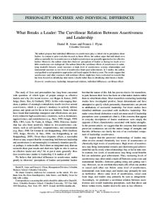
6. Appendix B: Homogeneous Assets, Concentrated Ownership: For the case of uniform distribution, the expected surplus (de…cit) turns out to be decreasing in for all 1 4 > 0 : The expected de…cit as a function of is given by S( ) = Ev [S(v1 ; v2 ; )] = 32 2 56 ; and 6 is depicted in Figure 1:

0 -0.2 0

0.5

1

1.5

2

-0.4

Deficit

-0.6 -0.8

Deficit

-1 -1.2 -1.4 -1.6 -1.8 Alfa

Figure 1: Surplus (De…cit) with Uniform Distribution

However, as our earlier discussion alluded to, in general, expected surplus can be non-monotonic when < 1. An example where this holds is as follows: Suppose that both agents’ valuations are distributed according to

F (v) =

8 > > < > > :

2v

v

1 2 (1 )v v (1

)v v

(1 2 ) 1

+

+1

1

2v if v if v 2 [ 2 v; v] :

if v

For this scenario the derivative of expected surplus with respect to as goes to 0.12

v

converges to v(1

(1 2

)

(1

)) > 0

7. Appendix C: Homogeneous Assets, Dispersed Ownership: Substitutes Here we show that the surplus (or de…cit) can be non-monotonic even in symmetric environments. Suppose that both agents are symmetric and their valuations are distributed on [0; 1] according to F (vi ) = vip ; for 0 < p < 1: 12

Details of the calculations for this example are available upon request.

28

(23)

We study how the parameter p (which determines how concentrated the distribution on small values is) a¤ects the threshold level of needed to achieve e¢ ciency.13 For this family, there is a cuto¤ value of above which e¢ ciency is possible, which is increasing in p. For example, for p = 0:5, this cuto¤ is 0:6; whereas for p = 0:25; the cut-o¤ is 0:41. In the following …gure, we graph the expected surplus for p = 0:01, and for p = 1 (the uniform case) and p = 10:

0.06

0.0005

0.2

0.04 0.0004

0.15

0.02 0

0.0003

0.1

0

0.1

0.2

0.3

0.4

0.5

0.6

0.7

0.8

0.9

1

-0.02 0.0002

0.05

0.0001

-0.04 -0.06

0 0

0 0

0.1

0.2

0.3

0.4

0.5

0.6

0.7

0.8

0.9

0.1

0.2

0.3

0.4

0.5

0.6

0.7

0.8

0.9

1

-0.08

-0.05

1

-0.0001

-0.1 -0.12

-0.1 al f a

al f a

al f a

p=0.01

p=10

p=1

: The graphs highlight the non-monotonicity of the surplus in ; whenever 1. We can see that as p grows, and high valuations become more probable, there is a higher threshold value for , above which e¢ ciency is possible. Higher valuation, which makes an agent less likely to be willing to part with his object, makes e¢ ciency more di¢ cult. There a higher increases S because it increases the willingness to pay for the asset.

8. Appendix D: Homogeneous Assets, Dispersed Ownership: Complements Example: Expected Surplus (or De…cit) can be Non-Monotonic in Asymmetric Environments. Consider an environment with distributions Fi (x) = xpi in [0; 1]. It is easy to see that vi = ( 2pj +1 + 1) 1=pj and @vi 2pj +1 + 1) 1=pj 1 p 1 (2p + 1) 2pj . j j @ = ( Fix > 1; but close to 1, and take p1 ! 0 and p2 ! +1. Then, with probability close to 1, v2 v1 and, moreover, F2 (v1 ) = 1=( 2p2 +1 + 1) 0, but F1 (v2 ) 1=2. Therefore, only two cases appear with 13

When both agents’valuations are distributed according to (23), the expected surplus is

S( )

=

2

Z

vdF

2

=

v p+1

p

dF

2

0

v

p 2 p+1

Z1

p+1

(1

v

Z

v p+1

p

dF + f1 +

p

g

0

p+1

)

p 4 2p + 1

where v satis…es 1 = ( v )p + ( v )p .

29

v p+1

+ (1 +

p

p ) (1 p+1

Z1 v

vdF 1

p+1 p+1

);

probability bigger than , both of them close to 12 :

S(v1 ; v2 ; ) = (1 + )v1 S(v1 ; v2 ; ) =

v2

v1

v1 if v1

v2 if v1

v2 and v1

v2 and v1

v2

v2 :

Then, we have @ S( ) = @

Z1

v1 f1 (v1 )dv1

v @v1 + 2 + @ 2

1 @v2 : 2 @

v2

Noting that the …rst three terms are bounded by one, but that @ S( ) < 0. @

@v2 @

goes to minus in…nity, we see that

References [1] Boone A. L. and J. H. Mulherin, (2007): “How Are Firms Sold?,” Journal of Finance, vol. 62(2), 847-875. [2] Borgers, T. and P. Norman, (2009): “A Note on Budget Balance under Interim Participation Constraints: The Case of Independent Types,” Economic Theory, 39, 477-489. [3] Brusco, S., Lopomo, G., Robinson, D. T., and S. Viswanathan, (2007): “E¢ cient Mechanisms for Mergers and Acquisitions,” International Economic Review, 48, 995-1035. [4] Clarke, E. (1971): “Multipart Pricing of Public Goods,” Public Choice, 2, 19-33. [5] Cramton, P., R. Gibbons, and P. Klemperer(1987): “Dissolving a Partnership E¢ ciently,” Econometrica, 55, 615-632. [6] Fang, H.M. and P. Norman, (2008): “Overcoming Participation Constraints,” Yale and UNC. [7] Figueroa, N. and V. Skreta (2011): “Asymmetric Partnerships,” mimeo NYU and Universidad de Chile. [8] Groves (1973): “Incentives in Teams,” Econometrica, 41, 617-631 [9] Jackson, M. and H. Sonnenschein (2007): “Overcoming Incentive Constraints by Linking Decisions,” Econometrica, 75, 241-257. [10] Jehiel, P. and A. Pauzner (2004): “Partnership Dissolution with Interdependent Values,”RAND Journal of Economics, 37, 1-22. 30

[11] Krishna, V., and M. Perry (2000): “E¢ cient Mechanism Design,” working paper. [12] Makowski, L. and C. Mezzetti (1993): “The Possibility of E¢ cient Mechanisms for Trading an Indivisible Object,” Journal of Economic Theory, Vol. 59, p. 451–465. [13] Makowski L. and C. Mezzetti (1994): “Bayesian and Weakly Robust First Best Mechanisms: Characterizations,” Journal of Economic Theory, 64, 500-519. [14] McAfee, R. P. (1991): “E¢ cient allocation with continuous quantities,” Journal of Economic Theory, 53,51-74. [15] Myerson R. B. and M. A. Satterthwaite (1983): “E¢ cient Mechanisms for Bilateral Trading,” Journal of Economic Theory, 29(2):p. 265–281. [16] Neeman, Z., (1999): “Property Rights and E¢ ciency of Voluntary Bargaining under Asymmetric Information,” Review of Economic Studies, 66, 679-91. [17] Schmitz, W. P. (2002): “The Coase Theorem, Private Information, and the Bene…ts of not Assigning Property Rights,” European Journal of Law and Economics, Vol. 11 (1), 23-28. [18] Schweizer, U. (2006): “Universal Possibility and Impossibility Results,” Games and Economic Behavior, 57, 73-85. [19] Segal, I and M. Whinston (2010): “A Simple Status Quo that Assures Participation (with Application to E¢ cient Bargaining),” forthcoming, Theoretical Economics. [20] Vickrey, W. (1961): “Counterspeculation, Auctions and Competitive Sealed Tenders,” Journal of Finance, 16, 8-37. [21] Williams S. R. (1999): “A Characterization of E¢ cient, Bayesian Incentive Compatible Mechanisms,” Economic Theory, Volume 14, Issue 1, p. 155 - 180.

31