Word Embeddings for Speech Recognition Samy Bengio and Georg Heigold Google Inc, Mountain View, CA, USA {bengio,heigold}@google.com
Abstract Speech recognition systems have used the concept of states as a way to decompose words into sub-word units for decades. As the number of such states now reaches the number of words used to train acoustic models, it is interesting to consider approaches that relax the assumption that words are made of states. We present here an alternative construction, where words are projected into a continuous embedding space where words that sound alike are nearby in the Euclidean sense. We show how embeddings can still allow to score words that were not in the training dictionary. Initial experiments using a lattice rescoring approach and model combination on a large realistic dataset show improvements in word error rate. Index Terms: embeddings, deep learning, speech recognition.
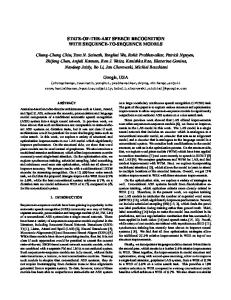
1. Introduction Modern automatic speech recognition (ASR) systems are based on the idea that a sentence to recognize is a sequence of words, a word is a sequence of phonetic units (usually triphones), and each phonetic unit is a sequence of states (usually 3). Linguistic expertise is then used to transform each word of the dictionary into one or many possible phonetic transcriptions, and one can then construct a graph where the nodes are states of these phonetic units, connected to form proper words, such that the best path in the graph (according to some metric) corresponds to the best sequence of words uttered for a given acoustic sequence [13, 17]. The basic ASR architecture is shown in Figure 1.
Figure 1: Architecture of a modern ASR system. The total number of unique states can vary depending on the task, but is usually very high. In our experimental setup, it is around 14,000. The best ASR approaches nowadays use
deep architectures [3, 4, 6, 8, 14] to estimate the probability of being in each state at every 10ms of signal, given a surrounding window of acoustic information. This usually means training a neural network with a softmax output layer of around 14 thousand units. Such a neural network is trained from data aligned using a previously trained model used to force-align the training sentences to states, that is, estimate for each time frame which state the model should be in, in order to produce the right sequence of states, hence the right sequence of words. We propose in this paper to replace the basic ASR architecture (the shaded box in Figure 1) with a suitable deep neural network. This leads to fully data-driven approach that avoids the rigid model assumptions of (3-state) HMMs (including the frame independence assumption) and does not require any linguistic expertise through the lexicon or phonetic decision tree [17]. On the down side, jointly learning all these components from data is a very hard learning problem. However, we argue that the original task in Figure 1 may be harder than the final task of recognizing word sequences: indeed humans would usually fail to properly segment an acoustic sequence of words into phonetic units, let alone into states, as the boundaries between them are hard to assess. It is certainly easier for humans to segment such acoustic sequence into words instead. Moreover, training dictionaries often contain about the same number of words (tens of thousands) as there are states in the model, so it might actually be about as hard to train a model to distinguish full words rather than states. We present a first attempt at such a task in the next section, based on a deep convolutional architecture. While such a model would then require a special decoder (to account for the fact that words have variable duration), it can more easily be used as a second phase lattice rescoring mechanism: using a classical pipeline (based on phonemes and states), one can obtain, at test time, not only the best sequence of words given the acoustic, but the k-best such sequences, often organized as a lattice in the induced word graph. Each arc of the lattice can then be rescored using the proposed word-based model efficiently. One problem of a model directly trained on words is arguably to be able to generalize to words that were not available at training time. Using models based on states lets linguists arbitrarily construct new words, as long as they are made up of known phonetic units. We present in this paper an alternative construction, based on word embeddings, that can be used to score any new word for any acoustic sequence, and that hence can generalize beyond the training dictionary. Several researchers have been working on (partial) solutions toward a more data-driven approach and to automate and simplify the standard speech recognition architecture as depicted in Figure 1. A recent line of work includes segmental conditional random fields [18] with word template features [12, 5], for example. Just to mention a few, other exam-
ples include grapheme-to-phoneme conversion [2], pronunciation learning [15, 10], and joint learning of phonetic units and word pronunciations [1, 9]. We show in the experimental section initial results on a large proprietary speech corpus, comparing a very good statebased baseline to our proposed word embedding approach used as a lattice rescoring mechanism, which improves the word error rate of the system.
2. Model The classical speech recognition pipeline using a deep architecture as an acoustic model follows a probabilistic derivation: Let A = {a}T1 be an acoustic sequence of T frames at and W = {w}N 1 be a sentence made of a sequence of N words wn . We are thus looking for the best such sentence agreeing with the acoustic sequence: W ? = arg max P (W, A) = arg max P (A|W )P (W ) W
W
(1)
where we then decompose the prior probability of a sentence P (W ) into the product of the conditional probabilities of each of the underlying words as follows: P (W ) =
N Y
P (wn |w1n−1 )
(2)
n=1
for a sequence of N words, which is usually taken care of by a separate language model (often estimated by a so-called n-gram model on a very large corpus of text). For HMMs, the acoustic term decomposes into a series of conditionally independent state-based factors (Viterbi approximation): P (A|W ) =
T Y
p(at+k t−k |st )P (st |st−1 )
(3)
t=1
where k is a hyper-parameter representing the width of the input acoustic provided as input to the neural network, and the sequence of HMM states st follows the sequence of words wn in W . In order to use a neural network to model the emission term, we then rewrite it as follows: p(at+k t−k |st ) ∝
P (st |at+k t−k ) P (st )
(4)
where we ignore the p(at+k t−k ) terms since they are the same for all competing sequences of words, inside the argmax of Equation (1). The prior probability of each state P (st ) is usually estimated on the training set, and the term P (st |at+k t−k ) is estimated by a neural network (usually deep) that ends with a softmax layer over all possible states s. 2.1. A Deep Neural Network over Words Assuming a provided segmentation τ0N where τn corresponds to the last frame of word wn and τ0 = 0, one can rewrite Equation (4) in terms of words instead of states, as follows: � � N P wn |aτn Y 1+τn−1 P (W |A) P (A|W ) ∝ = . (5) P (W ) P (wn ) n=1 We ignore the P (A) term since it is the same for all competing sequences of words, inside the argmax of Equation (1). Furthermore, note that P (W ) here is estimated on the training set,
while P (W ) from Equation (2) is estimated on a large corpus of text. Here, P (wn ) is the prior � probability�of word wn estimated
n is the probability to on the training set, and P wn |aτ1+τ n−1 see word wn given the acoustic of the word, estimated by a deep architecture whose last layer is a softmax over all possible words of the training dictionary. As explained in the introduction, such a model can then be used easily in combination with a classical speech decoding pipeline, by adding a lattice rescorer which produces, for each test acoustic sequence, a lattice of several potential sequences of words, together with their expected start time and end time. One can� then rescore � each of the arcs of the lattice using the ratio of n and P (wn ) and output the best sequence in P wn |aτ1+τ n−1 the lattice accordingly. Unfortunately, this approach can only consider sequences made of words that were available at training time, which is often a subset of what is expected to be seen at test time. The next section considers an extension in order to solve this issue.
2.2. Word Embeddings The layer right below the softmax layer of a deep architecture trained to estimate P (wn |acoustic) usually contains a good compact representation of the input acoustic, such that a decision over which word it is can be made. We argue that this representation is such that two words that sound similarly will have a similar representation in this space. We call this layer an embedding layer, similarly to various embedding approaches that have been proposed in the literature, in order to represent words, images, etc. [11, 16], except that in the latter, words are nearby if they have similar meanings, while in the former words are nearby if they sound alike. Thus, we propose to train a separate deep architecture that will have as input some features extracted from the words (such as letters or features of them), and that will learn a transformation into the embedding of the corresponding word 1 . We used letter-n-grams as input features representing words, adding special symbols [ and ] to specify start and end of words, such that letter-n-gram [I] represents the word I, and letter-n-gram ing] represents a commonly seen end-of-word. We can actually extract all possible such letter-n-grams and keep the most popular ones, counting their occurrences over the training set. This can be done efficiently using a trie. We kept around 50,000 of them, and represented each word as a bag-of-letter-n-gram. As an example, the word hello is then represented as the set of features {h, e, l, o, [h, he, el, lo, o], [he, hel, ell, llo, lo], . . . }. As a sanity check, we trained a neural network to predict a word given its bag-of-letter-n-gram, and succeeded with around 99% accuracy, showing that this representation is often unique and rich enough. In order to train a mapping between letter-n-gram word representations and word embeddings obtained from the softmax model predicting words from acoustics, we use the deep architecture shown in Figure 2. The left block (Deep Convolution Network) is the learned transformation between an acoustic sequence and a posterior probability over words. We first train this block independently, as described in Section 2.1. After that, we fix its parameters and train a second block (Deep Neural Network, represented in two copies sharing their parameters in the figure), which takes as input the letter-n-gram representation of 1 A similar approach for representing rare words by their letter trigrams was used in [7]
3. Experiments We describe in this section an initial attempt at learning word embeddings suitable for automatic speech recognition. We first describe the dataset we used as well as the baseline model; then we describe the model we used to predict words given acoustic features; following this, we describe the model we used to be able to generalize to words unknown at training time; finally, we show word error rate results on a speech decoding task. 3.1. Dataset and Features
Figure 2: Deep architecture used to train word embeddings
a word and returns a real valued vector of the same size as the word embeddings from the left column. The model is trained using a so-called triplet ranking loss, similar to the one used in [16], where we randomly select an acoustic sequence from the training set, the word that we know it represents, and a randomly selected other word (dubbed WrongWord in the figure), and apply the following loss: L = max(0, m − Sim(e, w+ ) + Sim(e, w− ))
(6)
where m is a margin parameter to be selected (often set to 1), e is the word embedding vector obtained at the layer below the softmax of the Deep Convolution Network, w+ is the embedding representation obtained at the end of the Deep Neural Network for the correct word, while w− is the embedding representation obtained similarly for the wrong word; Sim(x, y) is a similarity function between two vectors x and y, such as the dot product. Training the Deep Neural Network with this loss tends to move the embedding representation of letter-n-gram near the embedding representation of the corresponding acoustic vector. In order to train such a model faster, we actually use the socalled WARP loss [16], which weighs every triplet according to the actual estimate of the rank of the correct word (w+ ), which has been shown to improve performance when measuring ranking losses such as precision-at-k. Using such a trained model, one can then compute a score between any acoustic sequence and any word, as long as one can extract letter-n-gram features from it. Empirical evidence that such an approach appears to be reasonable can be seen by examining the nearest neighbors, in the underlying embedding space, of the embeddings of some letter-n-gram. Table 1 shows examples of such neighbors. It can be seen that, as expected, neighbors of any given word arguably sound like it. In order to show that it also works for new words, the last example shows a target word (“chareety”) that does not exist, but its neighbors still make sense. Table 1: Nearest neighbor examples in the acoustically similar embedding space. Word heart please plug chareety
Neighbors hart, heart’s, iheart, hearth, hearted, art pleased, pleas, pleases, pleaser, plea plugs, plugged, slug, pug, pluck charity, sharee, cheri, tyree, charice, charities
The training set consists of 1,900 hours of anonymized, handtranscribed US English voice search and dictation utterances. Word Error Rate (WER) evaluations were carried out on a disjoint test set of similar utterances, amounting to 137,000 words. 3.2. Baseline Deep Neural Network The input for the baseline network is 26 contiguous frames (20 on the left and 5 on the right to keep the latency low) of 40dimensional log-filterbank features [8]. The log-filterbanks are computed every 10ms over a 25ms window. The network consists of eight fully connected rectified linear unit layers (socalled ReLUs) with 2560 nodes each, and a softmax layer on top with the 14000 states as the output labels. Such an architecture has been shown to reach state-of-the-art performance [6, 8]. 3.3. Description of the Acoustic Deep Architecture The training set contains a total of 48,310 unique words that were seen at least 4 times each in the corpus. Using a previously trained model, we obtain a training set aligned at the word level, which provides an estimate of where each word utterance starts and ends. Using this information we computed statistics of the length of words and found that more than 97% of word utterances were shorter in duration than 2 seconds. We thus decided to consider context windows of 200 frames of 10ms each. When a word was longer, it was cut (equally on both ends) while when a word was smaller, we filled the remaining ends with zeros, which corresponds to the mean feature value. We also considered filling the vector with the actual frames around the word, but results were slightly worse, presumably because the variability of the contexts around training set words was not enough to encompass the particular examples of the test set. The deep architecture used to predict a word given a sequence of 200 acoustic frames stacks the following layers: 1. a convolution layer of 64 units over blocks of 10 frames by 9 features; 2. a ReLU; 3. a max pooling layer of 4 by 4, with a stride of 2 by 2; 4. a mean subtraction layer over blocks of 3 by 3; 5. a convolution layer of 64 units over blocks of 10 frames by 4 features; 6. a ReLU; 7. a max pooling layer of 4 by 4, with a stride of 2 by 2; 8. a mean subtraction layer over blocks of 3 by 3; 9. two fully connected layers of 1,024 units using ReLUs; 10. a softmax layer over all 48,310 words of the training dictionary. The model was trained on 90% of the training set, for about 5 days on a single machine, using stochastic gradient descent
and a learning rate that was slowly decreasing during the process (this can be compared to the baseline model, which took one week on 100 machines to train). At the end of training, we used the remaining 10% of the training set to measure the performance of the model, which was 73% accuracy. This number is difficult to compare to other approaches as this does not correspond to any classical speech recognition task (since it assumes perfect alignment, during decoding). Nevertheless, given the high number of classes (more than 48,000), an accuracy of 73% seems quite good. Furthermore, this number includes errors such as homonyms which are impossible to set apart without the context and a language model. 3.4. Description of the Letter-N-Gram Deep Architecture As explained in Section 2, the previous model cannot be used in a speech recognition task unless it is known in advance that all words to be decoded were part of the training set dictionary, which is often not a realistic setting. For our experiments, although the training set contained 48,310 unique words, the decoder we used at test time contained 2.5 million unique words. Looking a posteriori at the test set for further analysis, we found that around 12% of the word utterances in the test set were not in the training dictionary. We thus trained a second model, as explained in Section 2.2, following Figure 2. The deep architecture used to represent a word from a sequence of letters into the word embedding space is as follows: 1. a layer that extracts all valid letter-n-grams from the word, from a total dictionary of 50,000 letter-n-grams;
where we blended results from both the initial decoder and the lattice rescorer by averaging their score. As can be seen, the embedding approach by itself gets worse performance than the baseline model, but when combined together, the result beats the baseline, either for beam sizes of 11 or 15. Although the differences in WER seem small, they are significant for this test set. Table 2: Word Error Rates for the three compared models, with two different values of the beam search parameter. Model Baseline Word embedding model Combination
WER beam=11 beam=15 10.16 9.70 11.2 11.1 10.07 9.59
It is interesting to analyze the kind of errors the proposed approach makes. Table 3 shows the top few such mistakes, as well as the number of times they actually happened. As can be seen, most mistakes are due to the language model and are somehow reasonable. As expected, many words expected to be decoded in the test set were not in the training dictionary; for instance, the test sentence acrostic poems including similes and metaphors contained the word acrostic which was not in the training dictionary but was in the much bigger decoder dictionary, and was properly decoded thanks to the letter-n-gram approach.
2. three fully connected layers of 1,024 units using ReLUs. We trained this model to optimize the loss described in Equation (6) where the embedding vector (e in the equation) was obtained from the acoustic representation of a word, w+ and w− were respectively the output of the letter-n-gram deep architecture for the correct and incorrect words. Incorrect words were selected randomly from the training set dictionary. The model was trained on 90% of the training set, for about 4 days on a single machine, using stochastic gradient descent and a learning rate that was slowly decreasing during the process. At the end of training, we used the remaining 10% of the training set to measure the performance of the model, which was 53% word accuracy. Comparing this number to the 73% word accuracy obtained by the first model, it is clearly worse, but on the other hand, this second model can now be used to score any word for any acoustic sequence, and not just one of the words of the training dictionary. Furthermore, when making a mistake, the selected words often have very similar phonetic sequences to the correct word, and one can hope that a full decoder using a language model should help disambiguate the errors. 3.5. Results and Discussions Equipped with the complete word embedding model, one can now use it for lattice rescoring, after a classical decoder has been applied to test sentences. Such a lattice can be obtained by selecting how large the beam should be at every stage of the decoder: the larger the beam, the bigger the lattice. We considered two such beams, 11 and 15, to see how it impacted the performance, measured in Word Error Rate (WER). Table 2 shows WER for three different approaches: the baseline model is the state-of-the-art deep neural network based speech recognizer; the Word embedding model shows the performance of the proposed approach; finally, we considered a combination approach,
Table 3: Top errors made by the proposed approach. Target it’s and
Obtained its in
okay five ’cause
ok 5 cuz
Count 167 52 50 43 26
Comment fault of the language model short words are harder to capture fault of the language model fault of the language model ’cause was not a word in the decoder
4. Conclusion Acoustic modeling for ASR systems have recently changed paradigm, from mixtures of Gaussians to deep neural networks. They have however continued to model states of an underlying hidden Markov model. We have revisited this assumption in this paper, proposing to directly model words using deep neural networks. This yields a latent representation of words where words that sound alike are nearby. Using this fact, we have shown how to extend this approach to model any word, even those that were not available at training time. We have then shown initial experiments on a large vocabulary speech recognition task, reporting improvements in word error rate when such an approach was used as a lattice rescorer in combination with a baseline. While the proposed approach can readily be used in classical speech recognition pipelines, a better solution would be to write a complete decoder that could completely remove the dependency with state-based systems. A naive implementation of such a decoder would be prohibitive, as it would have to consider all possible word durations, but with some word duration modeling, it is worth considering.
5. References [1] M. Bacchiani and M. Ostendorf. Joint lexicon, acoustic unit inventory and model design. Speech Communication, 29(2-4):99–114, 1999. [2] M. Bisani and H. Ney. Joint-sequence models for grapheme-to-phoneme conversion. Speech Communication, 50(5):434–451, 2008. [3] G. Dahl, D. Yu, L. Deng, and A. Acero. Contextdependent pre-trained deep neural networks for large vocabulary speech recognition. IEEE Transactions on Audio, Speech, and Language Processing, Special Issue on Deep Learning for Speech and Language Processing, 20(1):30– 42, 2012. [4] G.E. Dahl, D. Yu, and L. Deng. Context-dependent pretrained deep neural networks for large vocabulary speech recognition. In IEEE International Conference on Acoustics, Speech, and Signal Processing, ICASSP, 2011. [5] G. Heigold, P. Nguyen, M. Weintraub, and V. Vanhoucke. Investigations on exemplar-based features for speech recognition towards thousands of hours of unsupervised, noisy data. In IEEE International Conference on Acoustics, Speech, and Signal Processing, ICASSP, 2012. [6] G. Hinton, L. Deng, D. Yu, G. Dahl, A. Mohamed, N. Jaitly, A. Senior, V. Vanhoucke, P. Nguyen, T. Sainath, and B. Kingsbury. Deep neural networks for acoustic modeling in speech recognition: The shared views of four research groups. IEEE Signal Process. Mag., 29(6):82– 97, 2012. [7] P.-S. Huang, X. He, J. Gao, and L. Deng. Learning deep structures semantic models for web search using clickthrough data. In Proceedings of CIKM, 2013. [8] N. Jaitly, P. Nguyen, A. Senior, and V. Vanhoucke. Application of pretrained deep neural networks to large vocabulary speech recognition. In Conference of the International Communication Association, INTERSPEECH, 2012. [9] C. Lee, Y. Zhang, and J. Glass. Joint learning of phonetic units and word pronunciations for asr. In Conference on Empirical Methods in Natual Language Processing, EMNLP, 2013. [10] L. Lu, A. Ghoshal, and S. Renals. Acoustic data-driven pronunciation lexicon for large vocabulary speech recognition. In IEEE Automatic Speech Recognition and Understanding Workshop, ASRU, 2013. [11] T. Mikolov, K. Chen, G. Corrado, and J. Dean. Efficient estimation of word representations in vector space. In Proceedings of the Workshop at ICLR, 2013. [12] P. Nguyen, G. Heigold, and G. Zweig. Speech recognition with flat direct models. IEEE Journal of Selected Topics in Signal Processing, 4(6):994–1006, 2010. [13] L. Rabiner and B.-H. Juang. An introduction to hidden Markov models. IEEE ASSP Magazine, 3(1):4–16, 1986. [14] F. Seide, G. Li, and D. Yu. Conversational speech transcription using context-dependent deep neural networks. In Conference of the International Communication Association, INTERSPEECH, pages 437–440, 2011. [15] O. Vinyals, L. Deng, D. Yu, and A. Acero. Discriminative pronunciation learning using phonetic decoder and minimum classification error criterion. In IEEE International
Conference on Acoustics, Speech, and Signal Processing, ICASSP, 2009. [16] J. Weston, S. Bengio, and N. Usunier. Wsabie: Scaling up to large vocabulary image annotation. In Proceedings of the International Joint Conference on Artificial Intelligence, IJCAI, 2011. [17] S. Young, J. Odell, and P. Woodland. Tree-based state tying for high accuracy acoustic modelling. In ARPA Spoken Language Technology Workshop, 1994. [18] G. Zweig and P. Nguyen. A segmental crf approach to large vocabulary continuous speech recognition. In IEEE Automatic Speech Recognition and Understanding Workshop, ASRU, 2009.