Christoph Freudenberg–Tamás Berki–Ádám Reiff
A Long-Term Evaluation of Recent Hungarian Pension Reforms MNB Working Papers 2 2016
Christoph Freudenberg–Tamás Berki–Ádám Reiff
A Long-Term Evaluation of Recent Hungarian Pension Reforms MNB Working Papers 2 2016
The views expressed are those of the authors’ and do not necessarily reflect the official view of the central bank of Hungary (Magyar Nemzeti Bank).
MNB Working Papers 2016/2 A Long-Term Evaluation of Recent Hungarian Pension Reforms (A magyar nyugdíjrendszer közelmúltbeli változásainak hosszú távú értékelése) Written by Christoph Freudenberg*, Tamás Berki, Ádám Reiff Budapest, July 2016
Published by the Magyar Nemzeti Bank Publisher in charge: Eszter Hergár H-1054 Budapest, Szabadság tér 9. www.mnb.hu ISSN 1585-5600 (online)
*The author`s surname until 2015 was Müller.
Contents
Abstract
4
1. Introduction
5
2. Legal framework
7
2.1 Short history
7
2.2 Current rules
7
2.3 Recent pension reforms
8
3. Applied indicators
11
3.1 Macro indicators
11
3.2 Micro adequacy indicators
13
4. Model outline
13
4.1 The micro simulation model
13
4.2 The macro model
19
4.3 Demographic and macro-economic assumptions
23
5. Effects of recent pension reforms
27
5.1 Adequacy of the Hungarian public pension system
27
5.2 Cash balance of the Hungarian public pension system
37
5.3 Implicit liabilities of the Hungarian public pension system
45
6. Sensitivity
51
6.1 Sensitivity on economic assumptions
51
6.2 Sensitivity on demographic assumptions
54
6.3 Effect of the personal income tax reform and abolishment of contribution ceilings 57 7. Conclusion
59
References
61
3
Abstract
This paper studies the effect of Hungarian pension reforms between 2009-2012 on the adequacy and long-term fiscal stability of the Hungarian public pension system. For the adequacy analysis, we use a micro simulation model to project future initial pension levels relative to future gross wages. For the analysis of fiscal stability, we use a generational accounting-based macro model to forecast future yearly cash balances and calculate implicit pension liability (IPL) indicators. We find that major recent reforms have stabilized the public pension system until around 2035, but after this, mainly due to unfavorable demographic developments, we project increasing deficits that reach about 4% of GDP by 2060. JEL-code: H55. Keywords: Pension reforms, Sustainability of pension systems, Micro simulation.
Összefoglaló
A tanulmány a magyar nyugdíjrendszer 2009-2012 közötti változásainak a hatását vizsgálja a nyugdíjba vonuláskor kapott átlagos kezdőnyugdíjak szintjére, valamint az állami nyugdíjpillér hosszú távú fiskális helyzetére. A jövőbeli átlagos kezdőnyugdíjak bruttó átlagbérhez viszonyított arányát egy mikroszimulációs eljárással becsüljük meg. A rendszer fiskális stabilitásának vizsgálatakor pedig egy korosztályok közötti elszámolásra (generational accounting) épülő makro-modellel jelezzük előre a rendszer jövőbeli éves egyenlegeit, illetve az ezekből számítható implicit nyugdíjkötelezettség (Implicit Pension Liability, IPL) mutatókat. Az eredményeink szerint a közelmúltbeli főbb szabályváltozások körülbelül 2035-ig stabilizálták az állami nyugdíjpillért, ez után azonban, főleg a kedvezőtlen demográfiai folyamatok miatt, növekvő deficitszinteket jelzünk előre, amelyek 2060-ra elérhetik az akkori GDP 4 százalékát.
4
1. Introduction Public pension schemes across OECD countries are in a constant transformation process. This is especially true for Central Eastern European (CEE) countries, such as Hungary, for which the transition into a market economy in the 1990s brought about significant changes that also affected their public pension systems. For these countries, there are three common sources that will profoundly affect their pension landscapes over the next decades. First, labor market careers change. Before 1990, a typical career path was continuous employment. But with the transformation from a planned into a market economy, unemployment soared, and fragmented career paths became a common phenomenon. It is increasingly apparent that these broken employment histories will have important consequences for pension systems in the upcoming decades, as less beneficial working careers will translate into lower pension levels. This raises concerns about the future adequacy1 of pension benefits in Hungary – at least for those with segmented career paths. The second concern is that population of CEE-countries is aging rapidly. This is also true for Hungary, where the fundament of this demographic transformation was laid down in the 1990s by immensely dropping birth rates.2 These low fertility rates have not recovered until today. Obviously, the children who were not born during the last two decades will not become contributors and tax payers in future decades either. Additionally, Hungarians are also getting older. Life expectancy converges rapidly to the high levels observed in old EU member states. As a result of these two phenomena, Hungary – similarly to other countries – can expect a doubling of the old age dependency ratio until 2060. This demographic development puts a substantial pressure on the unfunded public pension scheme. In Hungary, recent reforms are an additional third factor behind the profound changes of the future pension landscape. In 2009, a gradual increase in the statutory retirement age from 62 to 65 years until 2022 was legislated. One year later the government rolled back from the three-pillar system – which was introduced in 1997/98 – by de facto eliminating the second (funded) pillar. As 97% of second-pillar public pension rights were re-nationalized and transferred into unfunded future pension entitlements, -some economists worry about the fiscal burden in the distant future – despite improving short-term fiscal conditions due to larger contribution revenues. The 2010 pension reform also introduced early retirement privileges to women with long contribution careers, which partially offsets the effect of the retirement age increase reform of 2009. Further, the pension act of 2011 closed early 1
We will give an exact definition for pension adequacy in subsection 3.2. Broadly speaking, it reflects to what extent pensions can substitute wages once a person retires. 2 See Eurostat (2015) and subsection 4.3.1 of this paper.
5
retirement channels for most other scheme members. Finally, some non-pension-related reforms also had an (unintended) impact on the long-term position of the public pension scheme: for example, the flat-rate personal income tax reform of 2011 affected the public pension scheme by increasing net earnings, the basis of pension benefit calculations. The goal of this paper is to evaluate the effect of these recent pension reforms, together with the changing labor market histories and demography, on the public pension system in the long run. We assess the pension performance from two perspectives: (1) pension adequacy and (2) long-term fiscal stability. For the adequacy analysis, we project future pension levels by gender and date of retirement for each cohort. With respect to the fiscal perspective, we show the development of future cash flows, similar to the Ageing Report of the European Commission (2015). Additionally, we also calculate measures for Implicit Pension Liability (IPL), which summarize the long-term position of public pension schemes in one single number. IPL figures receive a lot of attention on the international stage, as they have to be reported in European national accounts from 2017 onwards. In the late 1990s and early 2000s, there were many papers which evaluated the Hungarian pension system in a similar way (Kane and Palacios 1996, Benczúr 1999, Simonovits, 2001, Rocha and Vittas 2002, Orbán and Palotai 2005). However, very few comparable pension studies have been carried out more recently (Pension Roundtable 2009, European Commission 2012).3 The aim of this paper is to partially fill this gap in quantitative pension evaluations. We provide a first detailed evaluation of the reforms enacted since 2009. Our calculations are based on large micro data sets on the contribution history of Hungarian citizens. These allow us to draw a differentiated picture of future pension adequacy, and to evaluate the impact of recent reforms not only on macro aggregates, but also on the distribution of pension entitlements. The paper is structured as follows. Section 2 summarizes the current legal framework of the pension system, and details recent reforms whose impacts we study. The indicators that we use to measure pension adequacy and long-term fiscal stability are presented in section 3. Section 4 describes the model that we use for long-term projection: we start with the micro simulation model to project individual contribution careers, and continue with the dynamic cohort model which we use to estimate future fiscal indicators. Then we outline our main demographic and macroeconomic assumptions, under which we do our baseline calculations. Section 5 contains the main results regarding the effect of recent pension reforms on pension adequacy, on future aggregate cash balances and on implicit
3
An analysis of second pillar changes in CEE countries in general can be found in OECD (2012), chapter 3 as well as Égert (2012).
6
pension liability measures. In section 6 we demonstrate briefly to what extent our results are sensitive to the main assumptions. Section 7 summarizes the main findings.
2. Legal Framework 2.1 Short history The Hungarian public pension system has changed on several occasions since its introduction in 1929, mirroring the dynamic political and economic environment.4 During the Second World War, pension schemes in Hungary lost their assets, because of large-scale damages in real estate assets and years of hyperinflation. After this experience an unfunded pension system was introduced in 1952, whose coverage was gradually extended in subsequent years. Since the Security Act of 1975 nearly the whole Hungarian population, including self-employed and civil servants, is insured in the public pension system. A further milestone in the Hungarian public pension system’s history is the establishment of a threepillar system in 1997, following the recommendations of the World Bank.5 Besides the PAYG first pillar, a mandatory funded second pillar was introduced. Voluntary and occupational pension schemes served as the third pillar of the old-age provision. In the aftermath of the financial crisis, however, the Hungarian government – which was under the Excessive Deficit Procedure and thus faced tight budgetary pressures – de facto reversed the 1997 reform by eliminating the mandatory funded second pillar in 2010 before its full maturation. After this reform, PAYG first pillar pensions represent the only significant old-age income for a vast share of the population, while voluntary and occupational pension schemes remain marginal.6
2.2 Current rules The Hungarian first pillar pension scheme reflects a classical defined benefit system, and it is based on the initial pension formula presented in equation (1). The initial pension benefit 𝐵 depends on the number of service years (summarized by the accrual factor (𝐴𝑅)7 and on average indexed net earnings (𝐴𝑌𝐼) since 1988. The initial benefit is further corrected by two additional factors: the retirement
4
See Hirose (2011), p. 171. Many Central Eastern European countries introduced a three-pillar pension system in the late 90s. For an overview see e.g. Drahokoupil and Domonkos (2012), p. 285f. For a more detailed description of the motivations and the exact measures of the 1997 pension reform, see Augusztinovics et al. (2002). 6 See European Commission (2012), p. 81. 7 The accrual factor, due to its nonlinear nature, favours relatively short and long service histories. 5
7
factor (𝑅𝐹) and the pillar factor (𝑃𝐹). The retirement factor reflects decrements (or increments) for early (or late) retirement, relative to the mandatory retirement age.8 The pillar factor reduces the first pillar benefit of those who stayed in the three-pillar system after the 2010 reform; however, this is only relevant for a small proportion (less than 3%) of the contributors. 𝐵 = 𝐴𝑅 ∗ 𝐴𝑌𝐼 ∗ 𝑅𝐹 ∗ 𝑃𝐹.
(1)
In terms of pension indexation, benefits are annually adjusted by the expected change in the consumer price index (CPI). However, if the actual (ex post) CPI-change is larger than the expected one, then pensions are further increased by the difference between the actual and expected CPI. As no such correction is made when the actual CPI is lower than the expected one, in this system pensions, on average, grow faster than the CPI.9 Since 2011, the revenue side of the Hungarian first pillar pension scheme consists of “social contributory taxes”, which combine pension, health and labor market contributions and add up to a total of 37% of gross earnings. There is no explicit rule about the distribution of the social contributory tax revenue among pension funds and funds with non-pension related goals. In 2011-2012, 34% of gross earnings went to the pension fund. From 2013, this rate increased to 37%, as now health contributions (3% of gross earnings) are also regarded as revenue of the pension fund.
2.3 Recent pension reforms – an overview In this paper, we will analyze the effect of four recent pension reforms, all taking place in the aftermath of the 2008 financial crisis. This section describes these reforms in turn: the retirement age increase legislated in 2009 (labeled as “RA65”), the switchback reform of 2010 (labeled as “switchback”), the early retirement cuts legislated in 2011 (labeled as “cut ER”), and the 40-service-year rule for women, effective from 2011 (labeled as “40-sy rule”).10 2.3.1 Reform in 2009: increase in retirement age In Hungary, the financial crisis of 2008 led to a large international bailout loan in October 2008, with the aim to stabilize the country’s fiscal position.11 The conditions for this financial assistance package of 20 billion EUR by the IMF, World Bank and European Union included several pension-related
8
The mandatory retirement age is 62.5 years in 2015 for both genders, and a gradual increase to 65 years has been adopted until 2022. Since 2011 early retirement paths are effectively closed. See also subsection 2.3.1. 9 For a further discussion of pension indexations in our model, see section 6. 10 For a comprehensive overview of reforms enacted before 2009, see Augusztinovics et al (2002) as well as Orbán and Palotai (2005). 11 This bailout loan was fully repaid by April 2016.
8
measures.12 A key element of these was the adoption of a gradual increase in the statutory retirement age from 62 to 65 years, and a parallel rise in minimum retirement ages from 60 to 63 years by 2022. Pension indexation also changed from Swiss indexation (which adjusts outstanding pensions by the average of the price and wage indices) to price indexation.13 Furthermore, the 2009 reform tightened the eligibility criteria for early and disability retirement, eliminated pension increases in 2009 and the 13th month’s pension from 2010 onwards.14 2.3.2 The switchback reform of 2010 In 2010, with the aim to further ease the short-run fiscal pressure, Hungary reversed the three-pillar system established by the 1997 reform, and de facto eliminated the second (funded) pillar. Around 90% of the capital, which was accumulated between 1998 and 2010 by mandatory private pension funds, was transferred to the central budget.15 The new rules declared that:
New entrants to the pension system were automatically enrolled in the mono-pillar system from 2011 onwards.
Previous mixed-pillar participants were given the possibility to stay in the second pillar (and hence keep their private funds) by making a special opt-out declaration. But as conditions were unfavorable,16 only 3% of them – mostly young and high income earners – made this declaration.
Those switching back to the first pillar were entitled to a full first-pillar pension: their pillar factor in Eq 1 (𝑃𝐹) increased from its previous value of 0.75 to 1.17 Additionally, they received in cash the positive real returns of their second pillar accounts (i.e. the difference between their total account
12
For a more detailed description, see Simonovits (2011). To be more precise, during this reform a GDP growth-related indexation was adopted, in which higher GDPgrowth would have led to higher-than-CPI pension indexation. But in practice, pensions were indexed according to CPI changes in 2010 and 2011, and from 2012 onwards rules changed to the price indexation that we described in subsection 2.2. 14 See European Commission (2012), pp. 82. In this analysis, however, we only consider the effect of the retirement age increase. Hence we assume that these other changes (i.e. 13th month pension, stricter disability scheme access) were already effective in the “pre-reform scenario”. This approach allows us to evaluate the effect of the retirement age increase in isolation. 15 A special state fund, named “Pension Reform and Debt Reduction Fund” was created. This was largely used to debt reduction in 2011 16 At the time of decision, those who opted to stay in the second pillar declared that they agree not to accrue any further pension rights from the first PAYG pillar, despite the 24% employer’s contribution that was still channelled into this pillar. Later, in 2011, these rules were changed due to constitutional considerations – but by this time the switchback decisions were made and assets were transferred. According to the current rules, remaining mixed-pillar members can accrue pension entitlements in the first pillar. Another ex post change was that now these mixed-pillar members can only make further payments to their private pension funds on a voluntary basis, as all their mandatory contributions (employer’s and employee’s) are diverted into the first PAYG pillar from 2011. See amendments of Paragraph 1 of Annex 1 to Law LXXX of 1997. 17 During the three-pillar system, around 75% of contributions were paid to the first pillar, and 25% to the funded second pillar. The pension formula factor 𝑃𝐹 reflected this proportion (𝑃𝐹 = 0.75). But with the switchback, the second pillar’s accumulated assets were transferred to the first pillar, and hence this pillar factor was changed to 𝑃𝐹 = 1 for all members who switched back. 13
9
value and their total contributions). 97% of previous mixed-pillar members, with a total accumulated wealth of 2.8 trillion HUF (10% of GDP), returned to the mono-pillar system.18 The government justified this switchback reform along two lines of reasoning. First, the transition costs of the gradual introduction of the second pillar19 were seen too high: the size of necessary central government transfers (to cover “missing” contributions that were diverted to private schemes) increased steadily from 0.19% in 1998 to 1.14% of GDP in 2010.20 Second, the investment performance of the privately managed pension funds was poor: in the 10 years before the reform (2000-2009) the average internal rate of return of second pillar assets (5.1% annually) was lower than the average inflation rate (5.6%).21 The 2010 reform also introduced early retirement privileges for women with long contribution careers. From 2011 onwards all females with 40 or more service years were allowed to retire early without the usual pension decrements; we consider the effect of this change separately (see subsection 2.3.4). 2.3.3 Reform in 2011: closing of early retirement channels In 2010, early retirement and disability represented the major reasons to exit the labor market, and hence almost 30% of Hungarian pension beneficiaries were younger than the statutory retirement age of 62 years.22 Disability prevalence rates have been one of the highest across OECD countries in recent years: in 2008, for example, almost 12% of the working age population (aged 20-64) received a disability benefit.23 Against this background, the Hungarian government passed a new legislation in 2011 which closed a number of channels into retirement before the legal retirement age. Early retirement was completely abolished from 2013 onwards (with the exception of women with long contribution careers, see subsection 2.3.4). Disability was not regarded anymore as part of the pension system, but it was transformed into a separate disability provision. The same applies for rehabilitation benefits. The payment of existing 3rd category disability pensions (partially disabled) was also stopped after May 2012 unless the beneficiary requested a complex re-examination of his/her health status.24
18
Probably an important factor in this high rate of return into the mono-pillar system was the fact that those who did not show up to make any declarations, were automatically returned into the mono-pillar system. The time frame within which this declaration could be made was also relatively short (6 weeks). For further details of the switchback reform, see Simonovits (2011), p. 16. 19 During the transition period, around 25% of the contributions went into the second pillar, while all pension payments were to be fulfilled from the first PAYG pillar, and this created a continuous financing need. 20 See Hirose (2011), p. 192. 21 This period covers a massive drop of returns in 2008. In 2009, however, returns outweighed the fall of the previous year. See also Hirose (2011), p. 183f. 22 See also European Commission (2012), p. 83. 23 See OECD (2010), p. 61. 24 See also European Commission (2012), p. 83.
10
2.3.4 The 40-service-year rule for women The switchback reform of 2010 also introduced early retirement privileges for women with long contribution careers. From 2011, all women with 40 or more service years were allowed to retire early without the usual pension decrements. We investigate the effect of this change on future pension obligations separately.
3. Applied indicators To assess the long-term performance of the Hungarian public pension scheme we apply two sets of indicators: 1) macro indicators and 2) micro indicators. The macro indicators are mainly used to evaluate the fiscal long-term stability of the pension scheme, while the micro indicators are applied to measure the adequacy of future pension benefits.
3.1 Macro indicators Implicit pension liability (IPL) is a standard indicator to estimate unfunded promises made in public pension schemes. In the literature three main definitions of IPL are established:25
Accrued‐to‐date liabilities (ADL): these contain the present value of pensions to be paid in future years due to rights accrued until a current base year; no entitlements may be accrued after the base year – neither by present nor by future workers. Thus, it reflects the total obligations if one closes the pension scheme today.
Current workers and pensioners’ liabilities (CWL): in this case we assume that the pension scheme continues to exist until the last current contributor dies, but no new entrants are allowed after the base year. With this concept, not only ADL are covered, but also the present value of pension entitlements that will be accrued by current contributors in the future – due to their future contributions – is taken into account.
Open‐system liabilities (OSL): these also cover the present value of pensions accrued by new workers entering the respective pension scheme after the base year. In other words, it is assumed that the pension scheme will continue to exist for a relatively long time horizon.26
The three liability concepts differ with respect to the consideration of future pension accruals. The group of ADL takes into account pension rights accrued in past years, only. It is, therefore, most compatible with backward looking statistics. ADL will be a new mandatory figure of national accounts
25
See e.g. Franco (1995), Holzmann et al. (2004) and Kaier and Müller (2015). The range of options extends from including only children not yet in the labor force, to an infinite perspective. We apply an infinite perspective. 26
11
from 2017 onwards.27 It provides valuable information on the government obligations accrued-to-date as well as on the households’ unfunded pension wealth earned until today. The other two concepts extend ADL by pension entitlements earned in future years by current workers (CWL) and future workers (OSL). In order to calculate net liabilities, the present value of gross liabilities is confronted with pension assets of the respective group. The estimation of assets also differs with respect to the time horizon applied. For the net ADL calculations, only financial reserves of the respective pension scheme accrued until the base year are taken into account as assets. In Hungary, these assets are not substantial, so in this paper we report gross ADL figures (which is also net ADL). Net liabilities of the Open-system group (OSNL), on the contrary, also take into account future contributions (and possibly taxes) paid by current and future generations into the pension scheme; we will refer to these as the implicit assets of the pension scheme. The OSNL indicator is used in this study to measure the fiscal sustainability of the pension scheme. A limitation of the OSNL indicator is that it is relatively sensitive to the economic assumptions chosen, namely to the discount and the wage growth rate. To overcome this shortcoming we use the relative financing gap (RFG) as an additional fiscal stability indicator.28 The RFG relates the OSNL figure to the sum of future discounted GDP values. The RFG outlines the necessary immediate and durable adjustment of the pension budget to close the OSNL in percent of future annual GDPs. In other words, it reflects by how many percent of annual GDP benefits must be reduced or revenues increased to put the pension scheme on a sustainable foundation. By relating the ONSL not to the current but to the prospective GDP values, the future economic ability to close the financing gap is taken into account. Thus, the RFG features the same virtues as the so called S2 indicator used by the European Commission for overall public finances.29 IPL measures are valuable, as they summarize the fiscal position of a pension scheme in one single number. Thus, they can be used to study the impact of pension reforms on pension finances. Most policy makers are, however, not yet familiar with such aggregated figures and the underlying concepts. Therefore, we also report the standard indicator of annual cash flows. Similar to the Ageing Report of the European Commission, we demonstrate the development of aggregate expenditures and contributions in future decades. Information on yearly cash flows is valuable as they show “timing
27
See also European System of National and Regional Accounts (ESA2010), chapter 17. The same methodology is applied by the US OASDI Board of Trustees (2014). They do, however, not provide any name for this separate indicator. 29 In fact, the relative financing gap is methodologically akin to the S2 indicator. 28
12
effects”: one can calculate the size of deficits or surpluses of a fiscal system for any given future year. Thus, flow figures can indicate in which future years the fiscal pressure may become strongest.
3.2 Micro adequacy indicators The standard figure for adequacy analysis is the replacement rate (RR), which is the pension level relative to earnings. Usually, initial pensions are compared to the pre-retirement income of the pensioner. The idea is that the individual aims to (partly) replace former earnings. In our estimations we will not focus on this replacement role of the pension system. Instead, our aim is to measure pension levels relative to average earnings in the economy. With this, we can study to which extent public pensions (the main income source of elderly) can keep track with the earnings of the working population. Thus, we take an intergenerational perspective. The indicator used for this analysis is called the adequacy ratio, which is defined as the initial pension benefit of a new retiree in a future year relative to the average wage in the economy in this future year.
4. Model outline In this section we describe our modeling approach. The micro simulation model presented in subsection 4.1 estimates future initial pensions of new retirees, and from this it calculates the micro adequacy indicator. The macro indicators, as well as yearly cash flows, are calculated with a macro model that we describe in subsection 4.2. Finally, in subsection 4.3 we discuss the main macroeconomic and demographic assumptions that we use for our baseline calculations.
4.1 The micro simulation model In this subsection we describe the micro simulation approach we use to estimate future pension benefits. We focus on the calculation of first pillar old-age pensions, whose initial level is calculated by the formula given in equation (1) of subsection 2.2.30 The simulation is based on a large dataset which covers the contribution history of the entire Hungarian contributors’ population in the period 19972006 (about 5 million individuals). To approximate contribution histories before 1997, we use a much smaller representative dataset that covers about 8,500 individuals. We start the description of our approach by taking a closer look at the benefit formula. In general, the initial old-age pension level 𝐵 at a certain retirement age 𝑠 for gender 𝑔 in the future year 𝑓, accrued up to the base year 𝑏 = 2010 can be estimated by
30
The estimation of 2nd pillar pension benefits is outlined in section A of the online Appendix. For a more detailed description of the whole micro simulation model, see section D of the online Appendix.
13
𝑜𝑙𝑑,𝐴𝐷𝐿 𝐵𝑠,𝑔,𝑓,𝑏 = 𝐴𝑅𝑠,𝑔,𝑏 × 𝐴𝑌𝐼𝑠,𝑔,𝑓 × 𝑅𝐹𝑠,𝑔,𝑓 × 𝑃𝐹𝑠,𝑔,𝑏 ,
(2)
𝑜𝑙𝑑,𝑂𝑆𝑁𝐿 𝐵𝑠,𝑔,𝑓 = 𝐴𝑅𝑠,𝑔,𝑓 × 𝐴𝑌𝐼𝑠,𝑔,𝑓 × 𝑅𝐹𝑠,𝑔,𝑓 × 𝑃𝐹𝑠,𝑔,𝑓 .
(3)
During the estimation, the following four factors have to be considered:
AR: Accrual rates. In the accrued-to-date (ADL) approach, years accrued up to base year 𝑏 are taken into account. In the OSNL-approach, all years up to future year 𝑓 are considered.
AYI: Average yearly income earned since 1988 until the future year of retirement 𝑓 (revaluated to year 𝑓).
RF: Retirement factor, which reflects the pension increment/decrement valid in future year 𝑓 for gender 𝑔 and retirement age 𝑠.
PF: Pillar factor. It reflects whether a scheme member of age 𝑠 and gender 𝑔 participates in the first pillar only (𝑃𝐹 = 1) or also in the second pillar (𝑃𝐹 = 0.75). In the accrued-to-date (ADL) approach, status in the base year 𝑏 matters; but in the OSNL approach, status in the future year 𝑓 is considered.
In the next subsections we describe the calculation of these four terms in turn. 4.1.1 Calculation of average yearly income (AYI) For the calculation of average yearly income (AYI), earnings since 1988 are taken into account: 𝑇𝐼𝑠,𝑔,𝑓
𝐴𝑌𝐼𝑠,𝑔,𝑓 = 𝐷𝐶𝐼
𝑠,𝑔,𝑓
× 365.
(4)
In this expression, 𝑇𝐼 is the total net income earned during insurance period, and 𝐷𝐶𝐼 is the number of days covered by insurance. According to the pension rules, the variable 𝐷𝐶𝐼 covers only the contributory service time, i.e. periods of maternity leave, sick leave or unemployment benefits – for which no monetary contributions have been made – are not taken into account. The number of days covered by insurance (𝐷𝐶𝐼) variable is taken from the contribution data base for the years 1997 to 2006. For other years (1988-96 and 2007+), we estimate the 𝐷𝐶𝐼 with a regression, in a similar way to estimating total service times (for details, see subsection 4.1.2). The total net income (𝑇𝐼) variable contains all net income which is earned between 1988 and the future year of retirement 𝑓. We estimate 𝑇𝐼 with the following five steps:
14
1. Gross earnings from 1988 onwards. 31 For years 1997-2006, we take this variable from the large contributory data set. For other years (1988-1996, 2007+), we have to estimate gross earnings. During the estimation, we take the gender- and education-specific32 average gross earnings per working day, for each age. We call these average wage profiles.33 To estimate earnings in the period 1988-1996, we use the wage profiles calculated from the contributory data set for 1997. For years after 2007, we use the same profiles calculated for the year 2006. In both cases, we correct the wage profiles with the macro statistics of average wage growth (for 1988-1996 and after 2007). During the estimation of future and past gross wages of individuals we take into account – besides age, gender and education – the individuals’ relative income positions. We calculate these relative positions from their relative performance between 1997 and 2006, for which we have data. For each individual, we estimate the deviation of his/her gross wage from the respective gender-, age- and education-specific mean gross wage, and take the average of these deviations for the years 1997-2006. We assume that individuals will remain at this average relative income position forever. 2. Net earnings from 1988 onwards. Reference earnings in the pension formula are calculated in net terms. So in the next step we calculate net earnings from the estimated gross earnings. For this calculation, we use income tax and contribution rates, earned income tax credits (whenever it existed) and contribution ceilings of the respective years. With this approach, we can also evaluate the effect of various income tax-related policy measures (e.g. introduction of flat income tax rate, abolishment of contribution ceilings) on the level and distribution of future pensions. 3. Adding future wage growth. For each individual, we consider his/her future wage development until retirement. 34 In our simulations, future wages can increase via two
31
To be precise, we have data on contribution bases, thus we projected these contribution bases in the past and future. The decisive part of contribution bases are earnings. 32 Direct information on educational attainment – a main determinant of life-cycle income – is missing from the contributory database. We proxy this variable for each individual based on the available aggregate standard occupational classification (SOC) codes. First, education probability profiles are derived by aggregate SOC codes, age and gender from the labor force survey database (for the period 1997-2006). Second, these empirical probabilities (reflecting the probability of having a primary school, vocational school, high school or college degree) are implemented in the contributory database by using a randomization technique. For further details see Bálint et al. (2009). 33 For example, the average wage profile of women with high school is their average gross salary, calculated at each age between 20-70. We can estimate eight average wage profiles for each year in the contributory data set (two genders times four education types). 34 This means that we use the Projected Benefit Obligation (PBO) approach, and not the Accumulated Benefit Obligation (ABO) approach. The crucial difference between these two approaches is the treatment of future wage developments. In our approach (PBO), future wage developments – due to general wage growth or promotions – are taken into account. The ABO method neglects these future wage increases. If the pension
15
channels: we consider future general wage growths (see subsection 4.3.2 on macro assumptions), as well as the promotions over the individuals’ employment life-cycle. These promotions are estimated from the average wage profiles (i.e. average wages at each age) calculated in step 1. 4. Valorization of past income. The Hungarian first pillar pension scheme valorizes past earnings until the point of retirement with the general (net) wage growth in the economy. We do this valorization with the pre-retirement index factor 𝑣. The factor 𝑣𝑡,𝑓 cumulates the wage growth 𝑓−1 (𝑔) between year 𝑡 and the year before retirement 𝑓 − 1: 𝑣𝑡,𝑓 = ∏𝑖=𝑡+1(1 + 𝑔𝑖 ) if 𝑡 < 𝑓 − 1
(and 𝑣𝑡,𝑓 = 1 if 𝑡 = 𝑓 − 1). For individuals who are assumed to retire after the base year (2010), these pre-retirement index factors will be calculated using the assumptions on future wage growth rates (see subsection 4.3.2). As only a certain fraction of reference earnings is considered as an assessment base for the benefit calculations, we assume that degression brackets are wage indexed after 2013. 5. Calculating total income. The total income variable (𝑇𝐼) is calculated by summing up all valorized, net reference earnings from 1988 till the year before retirement 𝑓 − 1: 𝑓−1
𝑇𝐼𝑓 = ∑𝑧=1988 𝑣𝑧,𝑓 𝑤𝑧 ,
(5)
where 𝑤𝑧 is the net reference earning estimated for year 𝑧. 4.1.2 Calculation of accrual rates (AR) The accrual rate reflects the accrued service time of a contributor.35 In case of accrued-to-date (ADL) entitlements, only the service time earned until the base year (2010) is considered. For open-system calculations, however, the entire service time – up to the point of expected retirement – is taken into account. Data on service time is available for all taxpayers, who contributed at least one day in the period 19972006 in the contributory data set. For a small sample of individuals, we also have the number of service days for each year for the period 1958-1996. All other service day data needs to be estimated. For this estimation, we split the missing worker career information into two parts: (1) years before 1988 and (2) years after 1987 (i.e. years 1988-1996 and years after 2006). For the first period, we assume full
scheme under investigation will (most probably) exist until the end of the workers‘ careers, their future wage growths should be taken into account. Therefore we use the PBO approach, which is also consistent with Eurostat recommendations. 35 Currently, the accrual rate amounts to: (1) 33% after the first 10 service years; (2) +2% for each service year between years 11-25; (3) +1% for each service year between years 26-36; (4) +1.5% for each service year between years 37-40; and (5) +2% for each service year above 40 years. It was planned that a constant accrual rate of 1.65% will be applied from 2013. However, this legislated change in the accrual scheme was abolished before it could have taken effect in 2013.
16
employment for age groups 18-70. For the second period, we use a two-step, regression based approach which we will now describe in detail. In the first step of this approach, we simulate which individuals are working in the missing years after 1987 (extensive margin). 36 For the period 1988-1996 we estimate the following linear probability model for the dummy variable that individual 𝑖 is working in year (𝑤𝑜𝑟𝑘𝑖𝑡 ): 𝑤𝑜𝑟𝑘𝑖𝑡 = 𝛼 + 𝛽1 𝑤𝑜𝑟𝑘𝑖,𝑡+1 + 𝛽2 𝑤𝑜𝑟𝑘𝑖,𝑡+2 + 𝛽3 𝑤𝑜𝑟𝑘𝑖,𝑡+3 + 𝛽4 𝑦𝑒𝑎𝑟𝑡 + ∑8𝑗=5 𝛽𝑗 (𝑒𝑑𝑢𝑐𝑖 = 𝑗 − 4) + 𝛽9 𝑆𝑈𝑀𝑊𝐷9706𝑖 + 𝛽10 𝑆𝑈𝑀𝑊𝐷97062𝑖 + 𝛽11 𝑎𝑔𝑒𝑖𝑡 + 𝛽12 𝑎𝑔𝑒𝑖𝑡2 + 𝛽13 𝑎𝑔𝑒𝑖𝑡3 + 𝛽14 𝑎𝑔𝑒𝑖𝑡4 + 𝜇𝑖𝑡 .
(6)
As explanatory variables, we include three leads of the dependent variable, the education of the individual (as a category variable), the age of the individual, the total working days between 1997-2006 (both in a non-linear way), and year dummies. We run separate regressions for the two genders, and weight the observations of the small sample to mimic the age, gender and accumulated service year distribution of the large dataset. For the estimation of employment probabilities after 2006, we use a similar specification: 𝑤𝑜𝑟𝑘𝑖𝑡 = 𝛼 + 𝛽1 𝑤𝑜𝑟𝑘𝑖,𝑡−1 + 𝛽2 𝑤𝑜𝑟𝑘𝑖,𝑡−2 + 𝛽3 𝑤𝑜𝑟𝑘𝑖,𝑡−3 + 𝛽4 𝑦𝑒𝑎𝑟𝑡 + ∑4𝑒=1 ∑70 𝑎=18 𝛾𝑒𝑎 (𝑒𝑑𝑢𝑐𝑖 = 𝑒) × (𝑎𝑔𝑒𝑖 = 𝑎) + 𝜇𝑖𝑡 ,
(7)
where we have included lagged dependent variables to reflect the persistent nature of working statuses, and include a categorical age variable interacted with education levels to reflect the profile of being active on the labor market (for each education level) with respect to age. From these regressions, we can estimate for each individual 𝑖 the probability that he/she will be working (at least 1 day) in year 𝑡 . We simulate individual employment statuses based on these estimated probabilities. 37 As a result of this, each individual will have a simulated working status history. In the second step, we estimate the actual number of working days (𝑤𝑑𝑖𝑡 ) of those individuals, who have been simulated active in year 𝑡. To estimate these working days, we use the following regression: 𝑗−4
𝑤𝑑𝑖𝑡 = 𝛼 + ∑3𝑗=1 𝛽𝑗 𝑤𝑑𝑖,𝑡−𝑗 + 𝛽4 𝑦𝑒𝑎𝑟𝑡 + ∑8𝑗=5 𝛽𝑗 𝑎𝑔𝑒𝑖𝑡
36
+ 𝜇𝑖 + 𝜀𝑖𝑡 .
(8)
One may criticize the choice of only two statuses (zero and non-zero working days). The distribution of working days observed in the period 1997-2006, however, confirms this approach. In fact, the majority of contributors feature either zero contribution days (about 25 per cent) or a level of contribution days close to 365 (366) days per year (about 60 per cent). 37 For this, each individual draws a random number from the uniform distribution for each year 𝑡. If this random number is smaller than the estimated probability, then the individual will be working; otherwise he/she will be inactive.
17
According to this specification, the number of days worked depends on working statuses in the previous 3 years (as former inactive workers, who just enter the labor force, on average work fewer days), on age (in a non-linear way), and on time and individual fixed effects. This regression is estimated separately for genders and education levels from the contributory data set. With this method we can simulate the working days history of each individual, and therefore their total service time as well. Note that since the original data set contains total (contributory and non-contributory) service times, this simulation is for the total service time. For the estimation of average yearly income (AYI), we only need contributory service time (DCI, see subsection 4.1.1). By subtracting non-contributory service times – which we can estimate from average non-contributory service times by age in our data set – from the simulated total service times, we can obtain estimates of contributory service times (DCI), and hence we can estimate the average yearly income.38 4.1.3 Calculation of retirement factor (RF) If an individual chooses to retire later than the statutory retirement age (SRA), he/she is awarded by pension increments. This is reflected in the retirement factor. In the pre-reform scenario, these increments amount to 6% per year. So if an individual retires exactly at the SRA, then 𝑅𝐹 = 1; if he/she retires later, then 𝑅𝐹 is increased by 6% after each additional year. We also assume that early retirement is possible (at least under the 2010 rules) if more than 37 service years have been accrued. This is reflected in a smaller than unity retirement factor. Retirement one year before SRA leads to a decrease in the retirement factor by 3.6% (𝑅𝐹 = 0.964); while two years of early retirement results in a decrement level of 8.4% (𝑅𝐹 = 0.916). When necessary, we also take into account the special rules that apply for women since 2011: women with 40 or more service years can retire before the SRA without any decrement in their retirement factor. 4.1.4 Calculation of the pillar factor (PF) The pillar factor differs for single pillar members and mixed pillar members. For single pillar members, 𝑃𝐹 = 1; while for mixed pillar members it is only 𝑃𝐹 = 0.75.
38
Until 1998, years at higher education, military service or unpaid maternity leave are recognized as noncontributory service time. As we do not have data on these, we could not take these into account. However, this affects the relatively old cohorts only.
18
After the switchback reform of 2010, the pillar factor of the previous mixed pillar members who did not switch back to the first pillar will change. It depends on the total service time (𝑆𝑌 𝑡𝑜𝑡𝑎𝑙 ) accrued until the end of 2010 (𝑆𝑌 𝑡𝑖𝑙𝑙2011 ) and thereafter (𝑆𝑌𝑓𝑟𝑜𝑚2011 ), according to the following formula: 𝑆𝑌 𝑡𝑖𝑙𝑙2011 𝑆𝑌 𝑓𝑟𝑜𝑚2011 ) 0.75 + ( ). 𝑆𝑌 𝑡𝑜𝑡𝑎𝑙 𝑆𝑌 𝑡𝑜𝑡𝑎𝑙
𝑃𝐹 𝑠𝑤𝑖𝑡𝑐ℎ = (
(9)
4.1.5 Aggregation: calculating cohort- and gender-specific average initial pensions Applying the procedures that we described in the previous subsections, we simulate future individual career paths for all individuals in the large contributory data set, and calculate the initial pension benefit for each individual for all possible years of retirement. Then from these individual initial pensions, we calculate cohort- and gender-specific averages, by taking the simple average for each cohort for both genders. This way we have estimates of average initial pensions that individuals who were born, for example, in 1970, can expect if they retire in 2033, 2034, 2035, … 2040. We will use these cohort- and gender-specific average initial pensions – conditional on retiring in a given year – as inputs in the macro model, to estimate total pension obligations in the future years. 4.2 The macro model This subsection describes the projection approach with which we estimate future pension revenues and expenditures. The output of the micro simulation model, i.e. an estimate about future pension benefits is taken as an input for this. We devote a special emphasis on changes in old-age and disability retirement patterns, as these may considerably affect future pension finances. 4.2.1 The revenue side The key determinant of future pension revenues is future gross earnings, which is the contribution base (𝐶𝐵). We estimate these from the average wage profiles (defined in subsection 4.1.1 as the gender- and education-specific gross wages per working days, for each age) of the base year, by correcting it with the assumed productivity growth forecasts (see subsection 4.3.2). So the predicted contribution base of an active individual aged 𝑠, belonging to gender 𝑔 at any future year 𝑓 (relative to the base year 𝑏) will be 𝑒𝑥𝑝𝑒𝑐𝑡
𝐶𝐵𝑠,𝑔,𝑓
𝑓−𝑏
= [∑𝑗=0 (1 + 𝑤𝑔𝑗 )]𝐶𝐵𝑠,𝑔,𝑏 .
(10)
The actual revenue of the pension system is the contribution base multiplied by the contribution rate (which we denote by 𝜏). The difficulty is that – at least in the pre-reform scenario – not all individuals pay the same contribution rate into the first pillar pension scheme: mixed pillar members pay a lower
19
rate than single-pillar members. We can, however, calculate the average contribution of an active individual by using the average contribution rate: 𝑎𝑣𝑒𝑟𝑎𝑔𝑒
𝐶𝑠,𝑔,𝑓
𝑎𝑣𝑒𝑟𝑎𝑔𝑒
= 𝜏𝑠,𝑔,𝑓 𝑎𝑣𝑒𝑟𝑎𝑔𝑒
where this average can be calculated as 𝜏𝑠,𝑔,𝑓
𝑒𝑥𝑝𝑒𝑐𝑡
𝐶𝐵𝑠,𝑔,𝑓 ,
(11) 𝑠𝑖𝑛𝑔𝑙𝑒
𝑚𝑖𝑥𝑒𝑑 𝑚𝑖𝑥𝑒𝑑 𝑚𝑖𝑥𝑒𝑑 = 𝑝𝑠,𝑔,𝑓 𝜏𝑓 + (1 − 𝑝𝑠,𝑔,𝑓 )𝜏𝑓
, where
𝑚𝑖𝑥𝑒𝑑 𝑝𝑠,𝑔,𝑓 is the age- and gender-specific probability of participating in the mixed pillar system in future 𝑠𝑖𝑛𝑔𝑙𝑒
year 𝑓, 39 and 𝜏𝑓𝑚𝑖𝑥𝑒𝑑 and 𝜏𝑓
are contribution rates in future year 𝑓 for mixed and single-pillar
members, respectively. 𝑎𝑣𝑒𝑟𝑎𝑔𝑒
However, not all individuals will actually pay the average contribution 𝐶𝑠,𝑔,𝑓
we have just
calculated. To take into account that some individuals are not working in every year, we correct this average contribution by the probability of being a contributor, 𝑝𝑐𝑜𝑛𝑡𝑟𝑖𝑏 . These probabilities of course are age- and gender-specific, and we also allow them to be time-varying (so that we can model expected future changes in participation rates). Therefore, to obtain the unconditional cohort average 𝑎𝑣𝑒𝑟𝑎𝑔𝑒
of the contributions, 𝑐𝑠,𝑔,𝑓 𝑎𝑣𝑒𝑟𝑎𝑔𝑒
𝐶𝑠,𝑔,𝑓
(as opposed to average contribution conditional on being active,
), we weight the average contribution per individual by these contribution probabilities: 𝑎𝑣𝑒𝑟𝑎𝑔𝑒
𝑐𝑠,𝑔,𝑓
𝑎𝑣𝑒𝑟𝑎𝑔𝑒
𝑐𝑜𝑛𝑡𝑟𝑖𝑏 = 𝑝𝑠,𝑔,𝑓 𝐶𝑠,𝑔,𝑓
.
(12)
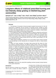
We assume that contribution probabilities will remain at their values observed in the base year (2010) for cohorts younger than 45 years. But for cohorts that are at least 45 years old, contribution probabilities will depend on four factors: (1) increase in legal retirement ages, (2) the cut in early retirement channels, (3) past retirement patterns, and (4) decreasing disability prevalence rates. Figure 1 shows the estimated age-specific contribution probabilities for males in 2010 vs 2025.40 In the next step, we account for the inaccuracies that stem from using micro data to calculate macro averages by calculating correction factors (𝜃𝑦 -s) for all years for which we have actual macro figures (2010, 2011 and 2012 in our case). These correction factors reflect the percentage by which the actual macro figure is bigger than the one calculated from the micro data set by aggregation: 𝜃𝑦 = ∑70
𝑇𝐶𝑦
𝑎𝑣𝑒𝑟𝑎𝑔𝑒
1 𝑖=20 ∑𝑗=0 𝑐𝑖,𝑗,𝑦
39
𝑃𝑖,𝑗,𝑦
,
(13)
This probability changed significantly with the switchback reform of 2010. A detailed description of our modeling approach to contribution probabilities can be found in section B of the online Appendix. 40
20
where 𝑃𝑖,𝑗,𝑦 is the population projection for year 𝑦 for the age cohort 𝑖 and gender 𝑗. For future years, we rescale the estimated total contributions (from micro data) with the most recent rescale factor (𝜃2012), to arrive at an estimate of the future macro figure. Figure 1. Contribution rates of males in 2010 and 2025 (estimated). Probability to be an active contributior in percent of the population
100% 90% 80% 70% 60% 50% 40% 30% 20% 10% 0% 20
25
30
35
40
45
50
55
60
65
age
2010
2025
without retirement probability
Finally, we calculate the total revenues of the first pillar pension scheme for any future year 𝑓 by aggregating the cohort- and gender-specific average contributions with weights taken from the population projection: 𝑎𝑣𝑒𝑟𝑎𝑔𝑒
1 𝑇𝑅𝑓 = ∑70 𝑖=20 ∑𝑗=0 𝜃𝑓 𝑐𝑖,𝑗,𝑓
𝑃𝑖,𝑗,𝑓 .
(14)
4.2.2 The expenditure side To calculate future expenditures of the first-pillar pension system, we take a similar approach as in the revenue side: first we calculate conditional (on being retired) average benefits, and then we multiply these conditional benefits with the probability of being retired to arrive at an unconditional estimate at the cohort level. In a final step we will just have to multiply these averages by the assumed size of the cohort (calculated from the demographic assumptions, detailed in subsection 4.3.1). Future pensioners can be divided into two categories: (1) those who are already retired in the base year (2010) (current retirees), and (2) those who will retire at a later point in time (new retirees).
21
For current retirees, estimation of their future pension benefits is relatively easy. We have information for the base year from the Hungarian pension authority (ONYF) on average pension benefit by age and gender (𝐴𝑃𝑠,𝑔,𝑏 ). From this, average pension benefits for the whole cohort 41 can be calculated as 𝑜𝑙𝑑 𝑏𝑠,𝑔,𝑏 = 𝐴𝑃𝑠,𝑔,𝑏 𝑅𝑠,𝑔,𝑏 /𝑃𝑠,𝑔,𝑏 , where 𝑅𝑠,𝑔,𝑏 is the number of 𝑠 year old pensioners of gender 𝑔 in the
base year, and 𝑃𝑠,𝑔,𝑏 is the total number of people in the same age cohort and gender. For new retirees, their average pension estimate (conditional on retiring in that year) comes from the 𝑛𝑒𝑤,𝑎𝑣𝑔 42 .
micro simulation model: average pension of new retirees at any future year 𝑓, is 𝐴𝑃𝑠,𝑔,𝑓
In a
second step, in order to calculate unconditional average pensions (for the whole cohort), we will multiply these average pensions by the probabilities that individuals of age 𝑠 and gender 𝑔 will actually 𝑛𝑒𝑤,𝑖𝑛𝑓𝑙𝑜𝑤
𝑜𝑙𝑑 retire in future year 𝑓, 𝑖𝑠,𝑔,𝑓 (the inflow rate into old-age pension): 𝑏𝑠,𝑔,𝑓
𝑛𝑒𝑤,𝑎𝑣𝑔
𝑜𝑙𝑑 = 𝑖𝑠,𝑔,𝑓 𝐴𝑃𝑠,𝑔,𝑓
.
The starting point in estimating these inflow rates and future retirement probabilities is observing retirement rates (by age and gender) in the base year. These current retirement probabilities are then transformed into future estimated retirement probabilities by taking into account three additional factors: (1) cohort-specific retirement histories (inflow rates) in the past; (2) legal changes (i.e. a change in the statutory or minimum retirement age should shift the retirement patterns in the future); and (3) future estimated net inflows into disability (those who get disabled will not become old-age pensioners in the future).43 As an illustration for the outcome of this procedure, Figure 2 depicts the current and estimated future (in 2016, 2022, and 2050) retirement probabilities for males, under the current pension rules.
Figure 2. Retirement probabilities for males in 2011, 2016, 2022 and 2050 (estimated).
41
Note that this way we are consistent with the calculations on the revenue side: we express all averages as unconditional averages, i.e. average in the whole population. 42 Note that this is the average pension of future new retirees in the single-pillar and mixed-pillar system: 𝑛𝑒𝑤,𝑎𝑣𝑔
𝐴𝑃𝑠,𝑔,𝑓
𝑛𝑒𝑤,𝑚𝑖𝑥𝑒𝑑
= 𝑝𝑚𝑖𝑥𝑒𝑑 𝐴𝑃𝑠,𝑔,𝑓 𝑠,𝑔,𝑓
𝑛𝑒𝑤,𝑠𝑖𝑛𝑔𝑙𝑒
+ (1 − 𝑝𝑚𝑖𝑥𝑒𝑑 ) 𝐴𝑃𝑠,𝑔,𝑓 𝑠,𝑔,𝑓
, where, like in subsection 4.2.1, 𝑝𝑚𝑖𝑥𝑒𝑑 denotes the 𝑠,𝑔,𝑓
probability that in a future year 𝑓, an individual of age 𝑠 and gender 𝑔 participates in the mixed-pillar system. 43 Ideally, retirement probabilities should also depend on individual characteristics (e.g. expected pension benefit, health status etc). We do not take into account these additional factors. For a more detailed description of the modeling of future retirement probabilities, see section C of the online Appendix.
22
100%
retirement probability per capita of the population
90% 80% 70% 60% 50% 40%
30% 20% 10% 0% 57
58
59
2011
60
61
62 retirement age
2016
63
64
65
2022
66
67
2050
Once we have these cohort-specific average benefits for current and future retirees, we can calculate 𝑜𝑙𝑑 𝑛𝑒𝑤 future average benefits starting from the base year’s data, 𝑏𝑠,𝑔,𝑏 and 𝑏𝑠,𝑔,𝑏 = 0, with the following
recursive formulae: 𝑝𝑒𝑛
𝑜𝑙𝑑 𝑜𝑙𝑑 𝑏𝑠,𝑔,𝑓 = 𝑏𝑠−1,𝑔,𝑓−1 (1 + 𝜋𝑓−1 ), 𝑝𝑒𝑛
𝑛𝑒𝑤,𝑖𝑛𝑓𝑙𝑜𝑤
𝑛𝑒𝑤 𝑛𝑒𝑤 𝑏𝑠,𝑔,𝑓 = 𝑏𝑠−1,𝑔,𝑓−1 (1 + 𝜋𝑓−1 ) + 𝑏𝑠,𝑔,𝑓
(15) ,
(16)
𝑝𝑒𝑛
where (1 + 𝜋𝑓−1 ) is the assumed pension indexation in the future year 𝑓 − 1 (in real terms). As a last step, we multiply these future, gender and age-specific average benefits at the cohort levels by the expected size of each cohort, and aggregate the results across cohorts and genders to arrive to an estimate for total expenditures of the first pillar pension scheme for the future year 𝑓, 𝑇𝐸𝑓 : 1 𝑜𝑙𝑑 𝑛𝑒𝑤 𝑇𝐸𝑓 = ∑100 𝑖=20 ∑𝑗=0(𝑏𝑖,𝑗,𝑓 + 𝑏𝑖,𝑗,𝑓 )𝑃𝑖,𝑗,𝑓 .
(17)
4.3 Demographic and macro-economic assumptions The results of our pension projection (in section 5) are very sensitive to the demographic and macroeconomic assumptions chosen. In this subsection we describe these assumptions in greater detail. 4.3.1 Demographic Assumptions and Demographic Developments
23
To ensure comparability to other country studies (e.g. European Commission 2014), we use Eurostat assumptions on the future development of fertility, mortality and migration. More precisely, we use the most recent demographic projection named EUROPOP2013. We consider alternative assumptions, including the one of the Hungarian Statistical Office (KSH), in the sensitivity analysis of section 6. Central Eastern European countries have experienced a rapid increase in life expectancy since 1990. In Hungary, life expectancy at birth rose by about 2.6 years per decade in the period 1990-2010 (see Table 1). According to EUROPOP2013, these recent positive trends in mortality are assumed to continue in future years, though at a slower pace. Until 2050 the life expectancy at birth is expected to rise by roughly 2 years per decade.44 After 2050 the increase amounts to roughly 1.5 years per decade. Total fertility rates have declined rapidly since 1990 and are currently among the lowest across Europe –in 2014 they were 1.34 births per women. According to EUROPOP2013 projections, total fertility rates are expected to increase over the next decades. Until the year of 2080, they converge to levels observed today in most other European Countries (see Table 1). Net migration, adding up to 0.15% of the population 2010, plays only a minor role in Hungary. EUROPOP2013 assumes relatively low net migration rates for future decades as well (see Table 1). Table 1: Main demographic determinants – a retrospect and outlook Hungary Actual Data
Demographic Projections - Europop2013
Year
1990
2000
2010
2020
2030
2040
2050
2060
2070
2080
Life Expectancy at Birth - males
65.2
67.5
70.7
73.6
75.9
78.1
80.1
82.0
83.8
85.4
Life Expectancy at Birth - females
73.8
76.2
78.6
80.2
82.1
83.8
85.5
87.0
88.4
89.7
Total Fertility Rate
1.87
1.32
1.25
1.5
1.61
1.68
1.72
1.74
1.75
1.76
Total Net Migration relative to the population
0.18%
0.16%
0.12%
0.25%
0.22%
0.25%
0.16%
0.15%
0.13%
0.12%
Source: own illustration based on Eurostat (2014).
Due to changes in the main demographic determinants (mortality, fertility and migration) the Hungarian population structure will change substantially in future decades. In this subsection we describe this demographic development in greater detail.45 We will focus on the timing of the ageing process, as it is essential to understand the changing fiscal pressure over the future decades.
44
It should be noted that there is a heated debate on the future development of life expectancy. Some advocate that the most reasonable assumption is to extrapolate past trends into the future (Oeppen and Vaupel, 2002, Wilmoth, 2000). Others oppose this idea and believe that there are biological limits to future life expectancy increases (Carnes et al., 2003, Carnes and Olshansky, 2007). Additionally, obesity is seen as a major obstacle to further increases in life expectancy (Olshansky et al., 2005). 45 The population projection is based on a program initially developed by Bonin (2001). The model has been updated to reflect the higher level of detail of the demographic assumptions provided by Eurostat.
24
In 2010, cohorts aged 50-60 were relatively large (see Figure 3).46 These cohorts are crucial for our pension projection, as they are expected to retire in the coming years. Cohorts aged 25-35 (the children of 50-60 years old baby-boomers) are also sizeable. Persistently low fertility rates in recent years led to relatively small young cohorts (aged 0-20) in Figure 3. The demographic structure of the base year 2010 has a huge impact on future population composition (see Figure 3). Figure 3: Structure of Hungarian Population in 2010/2030/2060 100 male
female
90 80
Age
70 60 50 40
30 20
10 0
100
80
60
40
20
0
20
40
60
80
100
Cohort Members (in 1000)
2010
2030
2060
Source: own calculations based on Europop2013 assumptions.
The old age dependency ratio (ODR) illustrates well the timing of the ageing process. It is defined here as the number of persons aged 65 and older, relative to the working population aged 20-64. In the past 20 years the ODR did not change substantially in Hungary. According to Table 2, the period of stable ODR has ended. Hungary is at the starting point of a new rapid ageing period: with babyboomers reaching retirement in the coming years, the ODR is expected to shoot up until 2025. After a short period of demographic stability in around 2025-2035, a second phase of rapid aging is expected. By 2060, the ODR is assumed to reach nearly 60% in Hungary, i.e. it is expected to double over the next 50 years. We stress, however, that demographic projections after 2030 should be interpreted with due care, as they are highly sensitive to the demographic assumptions. The demographic development until around 2030 is more reliable as it depends largely on the current population structure. Changes of the demographic assumptions and their impact on the fiscal projection are evaluated in section 6.2.
46
They have been born after World War II when fertility rates rose substantially in Hungary.
25
Table 2: The development of the age dependency ratio in EU28 and Hungary Year
1990
2000
2010 2015 2020 2025
2030 2035 2040
2045
2050
2060 2070 2080
Hungary
0.23
0.24
0.27
0.29 0.33
0.36
0.37
0.39
0.43
0.49
0.51
0.57
0.58
0.59
EU28
-
0.26
0.29
0.31 0.35
0.38
0.43
0.47
0.50
0.53
0.54
0.55
0.54
0.56
Source: own calculations based on Eurostat data.47
4.3.2 Macroeconomic assumptions The discount rate is one of the most crucial parameters for the calculation of pension liabilities. We apply a real discount rate of 3% over the projection horizon. This is in line with the assumptions applied by the European Commission (2014) and by Eurostat (2011). We also use the assumptions of European Commission (2014) for the returns of funded pension schemes. A 3% net rate of return (after asset management, contribution, account and annuity fees) is applied. Future wage growth is a further key parameter for the projection of pension systems. It has a decisive impact on both the revenue and the expenditure side of pension schemes. We assume that wage growth follows the recently published labor productivity growth forecasts of the European Commission (2014). According to these estimates, the Hungarian wage growth is expected to accelerate until 2030 and then to converge to a long-term average of 1.5% in real terms (see Table 3). GDP growth is estimated in our model based on wage and employment growth. In our calculations, employment rates depend only on changing retirement behavior. This means that we keep employment rates constant until the age of 45, as the main changes in employment rates are expected at higher working ages.48 Until 2030, GDP growth is assumed to add up to about 2% (see Table 3). Thereafter, a slowdown of GDP growth is expected as employment growth turns negative (due to the demographic developments). Table 3: Wage and GDP growth assumptions49 Year
2015
2020
2025
2030
2035
2040
2045
2050
2055
2060
Wage growth
4.3
1.4
2.1
2.2
2.1
2.1
2.1
1.9
1.7
1.5
GDP growth
2.9
1.9
2.1
2.0
1.5
1.2
1.3
1.4
1.2
1.0
Source: European Commission (2015)).
47
For years before 2001 we apply EU27 demographic data which are obtainable back to the year of 1995, only. According to the age-specific assumptions of the European Commission, the change in employment rates for cohorts aged between 20 and 44 in the period 2013-2060 is smaller than 5%. 49 In our baseline scenario, we use the European Commission (2015) assumptions, for the sake of comparability with other calculations. In its Growth Report of November 2014, MNB projects a higher GDP growth of 2.5% per year for the period of 2015-22, and the wage growth projection is also higher. In Subsection 6.1 we will show the impact of these alternative projections on the results. 48
26
5. Effects of recent pension reforms In this section we describe the effects of the recent four major pension reforms (detailed in section 2): the increase in legal retirement age of 2009, the switchback reform of 2010, the cut in early retirement channels of 2011, and the 40-service-year rule for women (effective since 2011). In order to provide a deeper understanding of their effects on the public pension system, we go step by step. First we show the effects of these reforms on the estimated level of future initial pensions (or the adequacy of newly awarded pensions), for which we use the micro simulation model described in subsection 4.1. Next, we present estimates on the changes in yearly cash balances, due to the reforms listed above. For these calculations, we use the macro model that was outlined in subsection 4.2. Finally, we summarize the effects of recent reforms in one single figure, by calculating the discounted sum of yearly cash balances. In particular, we report the effects on Accrued-to-Date Liabilities (ADL), Open-System Net Liabilities (OSNL) and Relative Financing Gaps (RFG). 5.1 Adequacy of the Hungarian public pension system This subsection reports the estimated effects of recent pension reforms on pension adequacy of the Hungarian public pension system. We mostly report gross adequacy ratios, i.e. gross initial pensions relative to gross average earnings in the economy (see also subsection 3.2). 50 Throughout this subsection, we define “initial pensions” as pension levels which are awarded to new retirees who retire exactly at the legal retirement age. Therefore changes which influence the timing of retirement, relative to the retirement age, are not reflected in these numbers. Our adequacy analysis covers entitlements earned in public pension schemes, namely first and second pillar pensions only. Other types of (voluntary) pension savings, which are of marginal nature in Hungary, as well as imputed rents or public in-kind benefits are neglected.51 We begin with presenting some facts about the most recent adequacy ratios, and estimated future adequacy ratios under the “pre-reform scenario”. Then we study the effects of the four reforms of section 2 one by one. Our starting point in the analysis of initial pensions is the pension formula, presented in equation (1) of section 3, which states that initial pensions depend on the number of service years (reflected in 𝐴𝑅, the accrual rate), on the average yearly income since 1988 (𝐴𝑌𝐼), on the retirement factor (𝑅𝐹) that
50
Note that net adequacy ratios are much higher than their gross pendants in Hungary, since pensions are tax free but salaries are not. 51 As presented by the OECD (2013), these other income sources can help to maintain living standards during retirement and may, therefore, be included in adequacy analysis. For Hungary, however, data on these resources is still limited.
27
includes decrements (increments) for early (late) retirement, and the pillar factor (𝑃𝐹 ) which is different for mixed-pillar members and single-pillar members. Our approach of considering initial pensions at the legal retirement age means the retirement factor will always be equal to one; therefore initial pensions reported here only depend on the three other factors.52 5.1.1 Adequacy of current public pension benefits53 Table 4 shows adequacy ratios of the Hungarian public pension system for the years 2007-2012. The top panel contains gross adequacy ratios for all existing pensioners (incl. a gender decomposition), while the middle panel reports the corresponding net adequacy ratios. The bottom panel shows the adequacy ratios of new retirees; this is the closest figure to those we estimate for the future years. 54 We can summarize the results as follows:
Current benefits of old age pensioners added up to about 42% of average gross earnings in the economy, and remained relatively stable during 2007-2012.
The net adequacy ratio is much higher: net pensions are approximately 66% of average net earnings in the years 2007-2012.
Similarly to earnings, there is a gender difference in pensions as well: male average benefits are about one third higher than their female counterparts.55
Benefits of new retirees are not much different from the entire pool of old age pensioners. They are, however, more volatile over time. This larger variance arises probably because of the frequent changes in pension rules, which led to large volatility both in the number and composition (in terms of socio-economic characteristics) of new retirees.
Overall, average gross initial benefits of new retirees in Hungary were lower than the EU average.56
52
Additionally, funded pension entitlements accrued in the 2 nd pillar also affect pension benefits. Their calculation is demonstrated in section B of the online Appendix. 53 Orbán and Palotai (2005), Pension roundtable (2009) and European Commission (2012) contain previous estimates on the adequacy of the Hungarian pension system. However, most of these estimates are limited as they do not differentiate by gender and other socio-economic characteristics, and none of these earlier studies evaluated the impacts of recent pension reforms. 54 Though it is not the same: recall that we will report adequacy ratios for new retirees who retire exactly at the legal retirement age, while the figures in Table 4 reflect the average adequacy of all retirees, irrespective of whether they retired early or in time (relative to the legal retirement age). 55 In calculating this figure, supplementary survivors’ pensions – which decrease the gap – were not taken into account. 56 For an EU comparison see European Commission (2012), p. 87. Note that the indicators used and the benefit types covered in EC (2012) are slightly differently defined: they report the initial pension relative to preretirement gross earnings (and not to average gross earnings) in the economy. This figure adds up to 38.4% for Hungary in 2010, which is about 10 percentage points lower than the EU average.
28
Table 4: Current adequacy ratios Adequacy ratio in gross terms ᵃ - all current old age retirees 2007
2008
2009
2010
2011
2012
Total
0.38
0.40
0.42
0.44
0.44
0.42
Males
0.46
0.48
0.51
0.53
0.53
0.49
Females
0.34
0.35
0.37
0.39
0.39
0.38
Adequacy ratio in net terms ᵇ - all current old age retirees Total
0.64
0.65
0.68
0.68
0.67
0.66
Adequacy ratio in gross terms ᵃ - new retirees 2007
2008
2009
2010
2011
2012
Total
0.49
0.39
0.43
0.47
0.47
0.46
Males
0.55
0.43
0.49
0.53
0.50
0.49
Females
0.42
0.32
0.36
0.40
0.45
0.45
a The adequacy ratio in gross terms is defined as average old age pensions in relation to average gross earnings in the economy b The adequacy ratio in net terms is defined as average old age pensions after taxes, if any, in relation to average net earnings in the economy
Source: Own estimates based on data provided by the ONYF. 5.1.2 Adequacy in the pre-reform scenario In Table 5 we present estimates on adequacy ratios of new retirees in the pre-reform scenario, which refers to the current legal situation without the four pension-related policy changes of section 2.57 According to our micro simulation-based projections, in the pre-reform scenario gross adequacy ratios would have remained relatively stable over time. The average initial pension of a male new retiree in future years, relative to the average earnings in the year of retirement, would have ranged around 42%. Women could expect slightly lower values of around 38%. It implies that the gender pension gap observed in recent data would have been expected to decrease over time. This is explained to a large degree by the use of a uniform retirement age of 62 in our calculations. In past years, women tended to retire earlier than men, and were more affected by early retirement penalties.
57
Hence, some measures that were taken simultaneously with the ones investigated here (like the abolishment of the 13th month pension, which was legislated at the same time as the retirement age increase from 62 to 65) are already taken into account in this pre-reform scenario.
29
Table 5: Adequacy ratio of an average scheme member - pre-reform scenario (incl. 1st and 2nd pillar, g=AWG, r_FDC=3%) 2012
2017
2022
2027
2032
2037
Males
0.45
0.41
0.40
0.41
0.41
0.43
Females
0.42
0.40
0.38
0.38
0.36
0.38
Source: own estimations. In order to explain why the adequacy ratio is predicted to remain roughly constant in future decades – despite significant changes in the labor market –, we decompose changes in the projected adequacy ratios in Table 6. Row 1 contains predicted adequacy ratios for the whole population – men and women together. Rows 2, 3 and 5 cover the change of each factor of the initial pension formula (see equation (1)): average accrual rates, average yearly incomes and average pillar factors. In addition, row 4 and 6 provide an estimate of the adequacy impact of 2nd pillar pensions.58 Finally, row 7 shows the estimated average education level of new retirees – to give an idea of the change in socio-economic characteristics that our calculations take into account. For the average accrual rate, our micro simulation predicts a significant drop for the upcoming decades. This is due to periods of unemployment and unreported employment emerging after 1990, which is in contrast to nearly full employment before 1989. As time goes by, new retirees’ will experience a gradually larger share of their employment career in this post-1990 era. These longer contribution records in post-communist times decrease the average total accrual rate of future retirees, by about 9% until 2037. Average yearly income (AYI) of future new retirees is presented in row 3 (in million HUF) without general earnings growth.59 Interestingly, this key parameter of the benefit formula does not change significantly over future decades. On the one hand, the gradual extension of the reference earnings to the entire working career should lower AYI over time. 60 On the other hand, however, future new retirees will be better educated (see row 7), which should increase AYI over time. The abolishment of contributions ceilings and the higher valuation of reference earnings in 2010-2012 (due-to the supergross rules of those years) should lead to higher AYI-s in future decades, too. The net effect of these
58
Note that by today this is no longer relevant, but in our pre-reform scenario most participants were mixedpillar members. 59 However, figures incorporate age specific promotions, career paths and individual education levels. 60 As discussed before, the AYI variable reflects the average net earnings since 1988. For new retirees in 2010, for instance, only the last 22 years of earnings are used for the calculation of reference earnings. For cohorts retiring later gradually the entire life-cycle earnings will be applied, which will also include relatively low earnings at the start of one’s working career. This fact should gradually decrease the AYI in future decades.
30
factors turns out to be almost zero in our calculations. In other words, the AYI is expected to remain relatively constant in future decades. Table 6: Drivers of pension adequacy, pre-reform scenario – example of individuals retiring at age 62 Retirement Year
2012
2017
2022
2027
2032
2037
Difference 2012 to 2037
Row 1
Average Adequacy Ratio ᵃ
0.43
0.40
0.39
0.39
0.38
0.41
-5%
Row 2
Total Accrual Rate
0.77
0.75
0.73
0.72
0.69
0.70
-9%
Row 3
Average Yearly Income (in mln. HUF) ᵇ
1.37
1.36
1.35
1.34
1.33
1.36
-1%
Row 4
FDC pension factor ᶜ
1.00
1.03
1.08
1.13
1.17
1.22
-
Row 5
Average Pillar Factor
0.99
0.95
0.90
0.87
0.86
0.84
-
Row 6
FDC net-effect factor ᵈ
0.99
0.97
0.97
0.98
1.01
1.02
3%
Row 7
Average education level ᵉ
2.42
2.49
2.51
2.56
2.62
2.67
10%
a Average adequacy ratio of both men and women b Inflation and real wage growth is neglected for reasons of comparison. c The FDC pension factor reflects the ratio of total public pensions (1st + 2nd pillar) relative to 1st pillar pensions. To ilsolate the different FDC effects, the pillar factor is set to one for this estimation. d The FDC net-effect factor multiplies the pillar factor with the FDC pension factor.
e Four education levels are considered to estimate the average education level, namely: Elementary degree = 1, Vocational degree = 2, High school degree =3 and College degree = 4.
Source: own estimations. As for the pillar factor (which makes the necessary correction for mixed-pillar members), there are again two factors that partially offset each other. On the one hand, the average pillar factor in the prereform scenario would have decreased over time. This can be seen in row 5. Under old rules participation in the second pillar was mandatory and the share of mixed-pillar members among the participants of the pension system would have increased gradually. As a consequence, the average pillar factor would have decreased over time. On the other hand, an increasing fraction of new retirees income would have come from private pension funds, i.e. the total pension of new retirees would have increased gradually relative to their first-pillar pension. These percentage increases are reported in row 4.61 The overall effect of the second pillar, which is the product of effects in row 4 and 5, can be seen in row 6. This second-pillar effect would have increased initial pensions by around 3% until 2037.
61
For example, those retiring in 2017 could expect (on average) a 3% increase in their initial pensions because of their accumulated private savings in the second pillar. In contrast, people retiring in 2037 would have had much more time to accumulate funds on their private accounts, so the contributions of their private savings to their overall pension would have been around 22%. These estimates are of course very sensitive to our assumptions about the future returns of private pension funds.
31
Overall, the compound impact of the different factors discussed (accrual rate, yearly income and FDC net factor) leads to a slight decrease in adequacy ratios over time in the pre-reform scenario. 5.1.3 The effect of retirement age increase to 65 Table 7 shows the estimated effect of the retirement age increase on future adequacy ratios. Qualitatively, this reform should increase adequacy, as by retiring later, new pensioners accrue more service years and probably have higher lifetime average income as well. Our results are in line with these expectations. Quantitatively, future new retirees can expect a rise in adequacy ratios by about 1 to 3 percentage points compared to the pre-reform.62 Table 7: Adequacy ratios after the increase in retirement ages Birth year
1950
1955
1960
1965
1970
1975
RA62 Scenario Retirement year Adequacy Ratio
2012
2017
2022
2027
2032
2037
Males
0.45
0.41
0.40
0.41
0.41
0.43
Females
0.42
0.40
0.38
0.38
0.36
0.38
RA65 Scenario Retirement year Adequacy Ratio
2012
2019
2025
2030
2035
2040
Males
0.45
0.42
0.42
0.42
0.43
0.46
Females
0.42
0.40
0.39
0.39
0.37
0.40
Source: own estimations. 5.1.4 The effect of the switchback reform in 2010 The switchback reform of 2010 influenced the pension entitlements of 3.1 million mixed-pillar participants (nearly every second Hungarian at working age 20-64). As discussed in section 2, these pension scheme members could either switch back to the mono-pillar system and give up all their previously accumulated assets in exchange for full future pension rights from the first pillar, or could stay in the mixed-pillar system. For many scheme members, including the relatively old ones who should not have entered the mixed-pillar scheme in 1998, staying in the mixed-pillar scheme was only
62
Our calculations reflect that a penalty free retirement can be realized under the new rules not until the age of 65. Under the RA62 scenario it was still possible to retire without decrements at the age of 62. Also, the effect of the retirement age increase depends on the number of service years accrued, due to the non-linear nature of accrual schedule. As most retirees have accrued between 26-36 service years, one extra year gives only a minimal increase of the accrual rate by 1%.
32
possible with relatively unfavorable conditions. Only 3% (about 97,400 individuals) of the previous 3.1 million mixed-pillar participants opted to stay in the mixed-pillar system.63 Before analyzing the effect of this switchback reform, we note two important factors that we did not take into account during the calculations. First, mixed-pillar scheme members accrued a 75% pension right from the state pillar, but this ratio does not reflect the exact proportion of their contributions into the state and private pension pillar. Initially, 8% employee contribution went to the private pillar and 24% employer contribution was paid to the state pillar, so the ratio of 75% was correct. But later, contribution rates changed frequently, and by 2010 the above contribution rates (going into the private and state pillar) were 10% and 27%, respectively. This means that the exact proportion, which mixed-pillar members should have accrued from the state pillar, was around 73% (=27/37) in 2010. As this “fair” proportion was changing – in parallel with the contribution rate changes – quite frequently between 1998 and 2010, we did not take into account these changes. Second, another important aspect that we do not consider in the analysis is the evolution of government debt during the transition from the initial mono-pillar system (in 1997) to the mixed-pillar system. While the introduction of the mixed-pillar system decreases the future burden on the state pillar for obvious reasons, it also leads to deficits during the transitory period: the reason is that while contributions are immediately channeled into the private pillar from the state pillar, pension payments only gradually decrease in the state pillar. In this analysis we do not take into account the costs of financing these transitory deficits. One can argue that if the deficits of the transitory period are financed entirely through increasing government debt, then we have to compare the future cost of this additional debt with the decrease in the future burden on the state pillar. But measuring the level of additional government debt due to transition into the mixed-pillar system is not straightforward, so we do not make this comparison. The rest of this subsection first investigates the effect of the switchback reform on the initial pension of previous mixed-pillar members (in Tables 8-9). Then we report adequacy ratios for all participants in the pension system (i.e. previous mono-pillar members and previous mixed-pillar members, in Table 10). Of course, our calculations are very sensitive to our assumption about the real return of private pension funds. To illustrate this sensitivity, we first report adequacy ratios under many alternative assumptions on the real return rate. Table 8 reports the adequacy ratios of average male and female mixed-pillar
63
Since then, the number of mixed-pillar scheme members decreased further due to some additional opportunities to switch back.
33
scheme members (“FDC members”) from different cohorts, before and after the switchback reform (in rows “No switchback” and “After switchback”, respectively). Of course, adequacy in the “No switchback” scenario depends crucially on our assumption on the internal rate of return of the private pillar, 𝑟𝐹𝐷𝐶 ; while in case of “Switchback”, adequacy does not depend on this rate. So different rows of the table report adequacy ratios in the “No switchback” case under different real return rate assumptions, and these numbers have to be compared with the numbers in the row labeled “After switchback”. To ease this comparison, red-marked cells indicate the cases when a stay in the mixedpillar system would have been better, for the average cohort member, than switching back to the mono-pillar system. If the rate of return of the private pension fund is 1% (or smaller), then for both genders and all cohorts, the average cohort members were better off by switching back to the monopillar system. For higher private pension fund returns, some younger cohorts would have benefitted if they stayed in the mixed-pillar system. If the assumed rate of return is 4%, for example, then all cohorts retiring later than 2025 would have benefitted from staying in the mixed-pillar system. The reason is that these scheme members, under large real returns, would have accumulated enough private pension rights (between 1998 and their retirement) to compensate for the lost first-pillar rights. But for older cohorts who retire earlier, even this relatively large real return rate would not have been enough to benefit from the mixed-pillar scheme. The reason is that these previous mixed-pillar members lose their private pension funds that they have accumulated since 1998, but in exchange they receive full public pension rights for their entire working career, which includes a significant service time even before 1998. Thus, the net effect of switchback is positive for them even when the real return rate is high.
34
Table 8: Adequacy ratios of mixed-pillar scheme members under different interest rate (r_FDC) assumptions
In the following, we analyze further the baseline case when the assumed real return rate is 𝑟𝐹𝐷𝐶 =3%. We chose this as the baseline as this is the real return rate that is commonly used in the literature, and this way our calculations are comparable with the literature. For previous mixed-pillar members (or FDC members), Table 9 compares their predicted adequacy ratios before and after the switchback reform. The top panel is the scenario before the switchback reform, and under the assumption of 3% real returns in the private pillar. The middle and bottom panels show the post-reform calculations, where we have calculated the figures for both subgroups: those who switched back (97%, middle panel) and those who stayed in the mixed-pillar system (3%, 35
bottom panel). Comparing figures in the middle and bottom panels, we see that under the new rules, previous mixed-pillar members gained (or at least did not lose) on average by switching back to the mono-pillar system for all cohorts that are due to retire before around 2035-2040, even under 3% real return rates in the private pension funds.64 This makes sense: those who retire relatively early, do not have enough time to accumulate enough wealth in their private pension accounts as a compensation for the lost pension rights from the first pillar.
Table 9: Adequacy ratios of FDC members - before & after the switchback reform Before the Switchback Reform 2015
2020
2025
2030
2035
2040
Males
0.52
0.50
0.53
0.54
0.54
0.55
Females
0.44
0.46
0.48
0.46
0.44
0.46
After the Switchback Reform Average FDC scheme member who switches back to the Mono-pillar System Males
0.59
0.54
0.53
0.51
0.48
0.47
Females
0.51
0.50
0.49
0.45
0.41
0.41
Average FDC scheme member who remains in the Mixed-pillar System Males
0.51
0.48
0.49
0.49
0.48
0.48
Females
0.44
0.44
0.45
0.43
0.40
0.41
Source: own estimations. In Table 10 we come back to our initial question of how the switchback reform of 2010 will affect future pension levels overall (i.e. not only for the previous mixed-pillar scheme members, whom we analyzed in Tables 8-9). Table 10 shows the adequacy ratios under the legal status quo of 2014 (i.e. it reflects the legislated rise in retirement ages to 65 as well as the impact of the 2010 switchback reform) on pension adequacy. The adequacy is shown for an average pension scheme member who retires at the age of 65. This scheme member is average in the sense that he or she is with a certain probability either a 1) previous non-FDC member; or a 2) previous mixed-pillar member who switched back to the monopillar system; or a 3) previous mixed-pillar member who remained in the mixed-pillar system. According to Table 10, adequacy ratios are slightly higher until 2030 due the switchback reform.
64
We note again that this statement is very sensitive to the assumed real return rates of private pension funds.
36
Thereafter, future new retirees are confronted with lower pension levels, as they cannot benefit from the higher interest gains of the FDC system. Still the impact of the switchback reforms on pension adequacy is limited. We note again that these results, in particular in the “Before switchback” scenario and in the long-run, are sensitive to the FDC interest rate assumption chosen. Table 10: Adequacy ratios (average of FDC + non-FDC members) before and after switchback 2015
2020
2025
2030
2035
2040
Before Switchback reform Males
0.44
0.42
0.42
0.42
0.43
0.46
Females
0.42
0.40
0.39
0.39
0.37
0.40
After Switchback reform Males
0.44
0.42
0.42
0.41
0.39
0.41
Females
0.42
0.41
0.40
0.38
0.35
0.37
Source: own estimations. 5.1.5 The effect of early retirement cut and 40-service-year rules The early retirement cut and the 40-service-year reform influence the timing of retirement, but not the initial pension level at the legal retirement age. Given our approach, in which we consider adequacy as the initial pension relative to gross earnings at the legal retirement age, these two reforms did not affect our adequacy measures. Their effects are considered in sections 5.2 and 5.3, when we study yearly cash balances and various measures of implicit pension debts on an aggregate level.
5.2 Cash balance of the Hungarian public pension system Now we turn to the estimated effects of recent pension reforms on yearly cash balances of the public pension system, which is based on a long-term projection of yearly revenues and expenditures. Reporting yearly cash balances is important for several reasons. First, these figures are easy to understand for policy makers and the wider public – relative to next subsection’s implicit pension liabilities. Second, cash flows are informative about the timing of fiscal pressure. Seeing these is especially important for reforms that may lead to short-term revenue gains (or losses) in exchange for higher (or smaller) government obligations in the more distant future. The aim of this subsection is to provide a better understanding of such long-term reform effects. We start this subsection by discussing the current cash balance and presenting the estimates for future cash balances in the pre-reform scenario. Then we turn to analyzing the effects of the four recent 37
pension reforms (RA increase, switchback reform, cut in early retirement channels and 40-service-year rule). Cash balance figures, presented in this section, cover public unfunded pensions, including old age, disability and survivors’ pensions.
5.2.1 Cash balance path in the pre-reform scenario The starting point of our pension projection is 2010, when the mismatch of total contributions and expenditures added up to 2.5% of GDP. With an exceptionally high contribution rate of 34% of gross earnings, total contributions amounted to 8.3% of GDP, while total pension related expenditures stood at 10.8% of GDP. Among the expenditures, 7.0% of GDP went to old-age pensions, 2.4% of GDP to disability pensions, and 1.3% of GDP to survivors’ pensions. The large share of total pension expenditures devoted to disability is explained by the high disability prevalence rates as well as by pension classification. 65 Benefits of disability beneficiaries beyond the legal retirement age are classified in disability in this study. In the pre-reform scenario we make a projection of future cash balances under the hypothesis that the four pension reforms to which we focus were not implemented. This means that we assume that (1) the statutory retirement age is 62 years; (2) roughly half of contributors participate in the mixed pillar system, with new entrants to the labor market being automatically enrolled into the 2nd pillar; (3) early retirement patterns are similar to those observed until 2010; and (4) women cannot retire penalty free with 40 or more service years acquired. The dotted lines of Figure 4 depict the predicted path of contributions and expenditures in the prereform scenario. In this case, gradually the entire Hungarian population would have participated in the mixed pillar system, channeling about one quarter of all contributions (8.5% of gross earnings) to the funded pillar. This is the main reason why contributions into the first pillar would have dropped from 9.2% of GDP in 2013 to 7.5% of GDP by 2040. The displayed increase in contributions in 2013 reflects the rise in employer contributions rates from 24% to 27% of gross earnings, which is considered in all four reform scenarios. The expenditures side, expressed relative to GDP, declines from about 11.6% in 2012 to around 9.5% in 2030 in the pre-reform scenario. Three factors can explain the expenditure drop until 2030: first, an increasing share of new retirees participates in the mixed pillar system. They have accrued fewer entitlements in the unfunded first pillar (i.e. PF=0.75 in equation (1)). Second, average benefit levels
65
See (OECD, 2010).
38
of new retirees are decreasing over time due to less beneficial contribution careers (see section 5.1, Table 6). As a consequence of these two factors, total old age expenditures would have decreased from 7.5% in 2012 to about 6.7% of GDP in 2030 despite the ageing of the Hungarian population. Third, overall pension expenditures drop due to a decline in disability expenditures. According to our estimates, in this pre-reform scenario total disability payments were expected to shrink by about 0.5% of GDP until 2020 and 1.0% of GDP until 2030, due to the more rigid eligibility criteria introduced earlier. After 2030 the disability pensioners’ population remains relatively stable and the development of overall expenditures is mainly determined by a changing number of old age pension recipients. In the period between 2030 and 2060, the old age dependency ratio is expected to rise substantially from about 37% to 57%. As a consequence of this rapid ageing process, total pension expenditures were expected to rise from 9.5% in 2030 to 11.4% of GDP in 2060 in the pre-reform scenario.66 Figure 4: Cash flows before and after the RA65 reform
Expenditures and Revenues relative to GDP
16%
14%
12%
10%
8%
6% 2010
2015
2020
2025
2030
2035
Expenditures - pre-reform
2040 2045 Year
2050
Expenditures - after RA65
2055
2060
2065
2070
2075
2080
Contributions - pre-reform
Contributions - after RA65
Source: own estimations. 5.2.2 The effect of retirement age increase to 65 The dashed lines of Figure 4 depict predicted contributions and expenditures after the implementation of the retirement age increase to 65 years. As expected, the RA65 reform lowers the mismatch of expenditures and contributions in future years. The effect of the reform to the contributions side is
66
The higher number of 2nd pillar members as well as the decline in average new pension benefits cushions the rise of pension expenditures also after 2030.
39
trivial: the increase in retirement ages translates into an extension of contribution careers. As a consequence, overall contributions are expected to increase by about 0.6% of GDP. On the expenditure side, however, delayed retirement has two effects with an opposite sign. First, the contribution period in which pension entitlements are accrued is prolonged by three years. This “entitlement effect”, ceteris paribus, increases future pension expenditures. But the general postponement of retirement will lead to a reduction in the number of future retirees.67 Ceteris paribus, this “postponement effect” lowers future pension expenditures. As shown in Figure 4, this postponement effect dominates the entitlement effect and long-term aggregate expenditures will decrease by about 0.6% of GDP relative to the pre-reform scenario.68 We can therefore conclude that the RA65 reform has improved the longterm stability of pension finances significantly: our estimates show that on average, the yearly cash balance improves by around 1.2% of GDP due to this reform. 5.2.3 The switchback reform of 2010 The marked lines of Figure 5 depict the yearly cash balances after the switchback reform of 2010. To ease comparison, we show additionally cash balances after the retirement age increase, but before the switchback reform (see dashed lines). The difference between the marked and dashed lines are due to the switchback reform of 2010. As it is apparent from Figure 5, the switchback reform stabilizes the public PAYG pension scheme until around 2030. Already in 2011, right after its legislation, total contributions increase by about 0.9% of GDP, as now (nearly) all contributors pay their entire pension contributions to the first pillar. This positive effect on the contribution side in the closer future is not as large as later on, since mainly younger cohorts with relatively low earnings were affected by the 2010 reform. In the long-run, however, the switchback reform is predicted to increase total contributions substantially, by around 1.3% of GDP relative to the pre-switchback scenario. On the expenditure side, the switchback reform shows almost no impact until around 2020. Most scheme members who retire before 2020 were not participating in the 2nd pillar. Hence their benefits, and consequently expenditures until 2020, are unaffected by the switchback reform. After 2020, however, an increasing share of new retirees participated in the second pillar until 2010. As a result, 67
Scheme members enter later into retirement. A smaller share of the population is therefore classified as retirees. A part of scheme members will not reach retirement anymore after the legal changes as they pass away between the age of 60 (old minimum retirement age) and 63 (new minimum retirement age). According to our estimations, about 5% of male and 2% of female scheme participants would have reached the old minimum retirement age but not anymore the new one in 2022 due to relatively high mortality rates in Hungary at the age of 60 to 62. 68 After the phase in of the RA65 reform, i.e. after 2022, the expenditure decline is smaller due to the entitlement effect.
40
their PAYG pension rights increase by one third (from 75% to 100%) relative to the pre-switchback scenario. Consequently, old-age expenditures start increasing as well, which leads to an enlargement of overall expenditures by 20% over the long-term. For 2060, we predict that expenditures rise by around 2.0% of GDP, relative to the pre-switchback scenario. We can, therefore, conclude that the switchback reform of 2010 eases the fiscal pressure in the PAYG system until around 2030 due to higher contribution inflows. After this, however, relatively high pension obligations (due to the switchback reform) will coincide with worsening demographic conditions. Figure 5: Cash flows before and after the 2010 switchback reform 15%
Expenditures and Revenues relative to GDP
14%
13% 12% 11%
10% 9% 8% 7% 6% 2010
2015
2020
2025
2030
2035
2040
Expenditures without Switchback
2045 Year
Expenditures with switchback
2050
2055
2060
2065
2070
2075
2080
Contributions without switchback Contributions with switchback
Source: own estimations. 5.2.4 The effect of early retirement cut in 2011 The dotted-dashed lines of Figure 6 depict projected contributions and expenditures, when we also take into account the cut in early retirement possibilities legislated in 2011. For comparison, we have added the predicted revenues and expenditures without this reform (but with the retirement age increase and switchback reform, see marked lines). Therefore, the difference between the dotteddashed lines and the marked lines on Figure 6 captures the effect of the early retirement reform only. The main message of Figure 6 is that the early retirement cut reform extends the period in which the current mismatch of contributions and expenditures turns into a budget surplus for 2020-2035. This positive development is mainly driven by an increase in revenues, due to the extension of contribution 41
careers. The postponement of retirement will reduce total pension expenditures by about 0.3% of GDP in the first two decades after its introduction. This positive postponement effect to the expenditure side is, however, gradually reduced by the entitlement effect, which arises because pension benefits of new retirees will be higher than under the pre-retirement cut scenario due to longer contribution careers. Additionally, disability expenditures rise due to the cut of early retirement. Under old rules entrance into disability was possible until the minimum retirement age. With the abolishment of the early retirement channel, however, disability is possible until the higher legal retirement age. Therefore, more individuals can be expected to become disability beneficiaries. On the very long run, overall expenditures are expected to increase by about 0.1% of GDP, as the entitlement effect and disability effect outweigh the postponement effect. We can conclude that the cut of early retirement channels further stabilizes the pension system over the next two decades. Figure 6: Cash flows before and after the early retirement cut reform
Expenditures and Revenues relative to GDP
15% 14% 13% 12%
11% 10% 9% 8% 7% 6% 2010
2015
2020
2025
2030
2035
2040 2045 Year
2050
2055
2060
2065
2070
2075
2080
Expenditures without early retirement cut
Contributions without early retirement cut
Expenditures with early retirement cut
Contributions with early retirement cut
Source: own estimations. 5.2.5 The effect of the 40-service-year rule In Figure 7, the circle-marked lines depict the contributions and expenditures if we additionally take into account the 40-service-year rule for women. Again, we added the same contribution and expenditure projections without the 40-service-year rule (see the dotted-dashed lines), so that one can see the effect of this particular reform separately. 42
The most important effect of the 40-service-year rule is that it increases projected expenditures and decreases projected contributions, so cash balances will deteriorate. We estimate that by 2013, about 30% of women can benefit from this new rule, and the proportion will gradually increase to about 35% in 2022 as more women reach 40 service years after the retirement age increase becomes effective. In the period 2022-2030 the proportion declines to about 25% due to less beneficial contribution careers (and remains at this level thereafter). In terms of quantitative estimates, we project a permanent drop in contributions of about 0.2% of GDP, due to shortened contribution careers of a large fraction of female contributors. On the expenditure side, an increase of about 0.3% of GDP is estimated; this is because women taking advantage of this rule can retire before the statutory retirement age without any pension penalty. The resulting longer retirement duration together with the absence of pension decrements increases expenditures. As a consequence, future yearly cash balances are expected to deteriorate by about 0.5% of GDP over the long run, when considering the 40-service-year rule. Figure 7: Cash flows before and after the 40-service-year reform 15%
Expenditures and Revenues relative to GDP
14% 13% 12% 11% 10% 9% 8% 7% 6% 2010
2015
2020
2025
2030
2035
2040 2045 Year
Expenditures without 40 service year rule Expenditures with 40 service year rule
2050
2055
2060
2065
2070
2075
2080
Contributions without 40 service year rule Contributions with 40 service year rule
Source: own estimations. 5.2.6 Summary of the four reforms Figure 8 shows together the effects of the four different pension reforms – all discussed above – on the yearly cash balances. To economize the number of projections on the figure, we only show the
43
cash balances (as opposed to showing separately the contributions and expenditures). The main conclusion about the overall effect of the recent reforms is mixed. On the one hand, the fiscal pressure on the pension system is significantly softened over the next decades. The retirement age increase, the switchback reform and the closing of early retirement channels will all lower the mismatch between contributions and expenditures until about 2045. The only exemption is the new early retirement channel for women with 40 service years, which increases the mismatch over the entire projection horizon. Still, the system seems to be relatively stable in terms of cash balances until around 2040.
Mismatch between Contributions and Revenues relative to GDP
Figure 8: Future mismatch of contributions and expenditures - after recent reforms 5%
4%
3%
1.
2%
2.
1%
0% 3. 4. -1%
-2% 2010
2015
2020
2025
2030
2035
2040 2045 Year
Pre-Reform Scenario … & after Switchback Reform … & after 40 service year rule (current rules)
2050
2055
2060
2065
2070
2075
2080
… after RA65 … & after Early Retirement Cut
Source: own estimations. On the other hand, the projection indicates an increasing mismatch between contributions and expenditures on the longer horizon, after 2040. The most important factor for this development is the rapid ageing process in the years between 2030 and 2060, when the old age dependency ratio is expected to rise by more than 50%. However, the 2010 switchback reform and the 40-service-year reform contribute to this increasing instability of pension finances after 2030 (while the other two reforms have positive effects). The switchback reform alone increases annual deficits by about 1% of GDP over the very long-run.69
69
We have to make it clear again that we do not take into account that the switchback reform decreased the government debt, and ceteris paribus led to smaller debt servicing costs in the future.
44
Considering all four reforms, the mismatch between contributions and expenditures, partly due to demographic reasons, is projected to increase to about 4% of GDP in 2060. In Table 11 we show the projected pension expenditures, revenues and imbalances until 2080 under the current rules (i.e. after all recent pension reforms). At the expenditure side, we distinguish between old age, disability, survival and other types of pension payments. Here we see again that the pension system is more or less balanced until around 2035, and deficits start to increase after 2035. As shown in Table 11, the deficit after 2035 is mainly driven by rising old age expenditures which increase due to demographics. Table 11: Projected pension expenditures, revenues and deficits after recent reforms70 (% of GDP) Expenditures Year
2010
2015
2020
2025
2030
2035
2040
2045
2050
2055
2060
2065
2070
2075
2080
Old age total
6.9
6.7
6.3
6.1
5.9
6.0
6.6
7.5
7.9
8.4
9.0
9.3
9.4
9.6
9.7
Disability total
2.4
2.4
2.3
2.2
2.1
2.1
2.2
2.3
2.3
2.4
2.5
2.5
2.5
2.6
2.6
Survivors' total
1.3
1.2
1.1
1.1
1.1
1.1
1.2
1.3
1.4
1.5
1.6
1.6
1.6
1.6
1.6
Other
0.2
0.3
0.2
0.2
0.3
0.3
0.3
0.3
0.3
0.3
0.3
0.3
0.3
0.3
0.3
Total pension expenditures (A)
10.8
10.6
9.9
9.7
9.3
9.5
10.3
11.4
11.9
12.6
13.4
13.7
13.9
14.2
14.2
9.7
9.7
9.7
9.6
9.6
9.6
9.6
9.6
2.9
3.7
4.1
4.3
4.5
4.6
Contributions Total pension contributions (B)
8.3
9.6
9.7
9.7
9.8
9.8
9.7
Imbalance of contributions and expenditures Imbalance = (A) - (B)
2.5
1.0
0.2
0.0
-0.4
-0.2
0.6
1.7
2.2
Source: own calculations.
5.3 Implicit liabilities of the Hungarian public pension system In this subsection we report implicit pension liability (IPL) figures, which reflect the sum of future discounted fiscal flows of a selected unfunded pension system. They summarize the findings of cash flow projections, presented in the previous section, in one single figure. In particular, we calculate the discounted sum of the projected future expenditures and cash balances, and the effect of recent reforms on these. As described in section 3, we use three approaches. First we use a gross-liability concept and provide ADL-estimates for Hungary. Then we also pay attention to net liabilities, and report OSNL-figures of the public pension system. Finally, we report the estimates of Relative Financing
70
The classification of different types of pension-related expenditures in Table 11 is somewhat different from the classification of official pension statistics. Here we classify disability pensions as benefits paid for those who ever received a disability benefit – irrespective of their age. This approach is convenient from a modeling point of view. In practice, disability pensioners who reach the legal retirement age and also apply for old-age pension, are re-classified as old-age pensioners.
45
Gaps, i.e. the permanent improvement in yearly pension balances that are necessary to close the OSNL figures to zero. There are several reasons why we provide estimates of both gross and net liabilities in this subsection. First, with this double focus we obtain a better understanding of the exact effects of recent pension reforms. We will see that ADL and OSNL figures might be quite differently affected. Second, unfunded pension rights represent by far the largest item of the households’ assets portfolio, and therefore the ADL figure itself is an important measure of Hungarian households’ wealth. Finally, we also focus on the ADL figure because from 2017 onwards it will be obligatory to report it in the new supplementary table of national accounts. In this subsection we start again by reporting the implicit pension liabilities (ADL and OSNL) in the prereform scenario. Then we consider the recent reforms one by one, and report their effects on the projected ADL and OSNL figures, and on the estimated RFG-s, too. 5.3.1 Implicit pension liabilities in the pre-reform scenario71 Figure 9 shows the projected implicit pension debts of Hungary in the pre-reform scenario. According to our projections, in 2010, accrued-to-date liabilities – which reflect pension rights earned until 2010 – added up to 252% of GDP. From the debtor’s (i.e. the government’s) perspective, this stock represents the overall implicit obligations arising from the general unfunded pension system. From the creditors’ (i.e. households’) view point, this figure can be interpreted as total unfunded public pension wealth. Currently this is not recorded in statistics, neither in households’ surveys nor in national accounts. Nevertheless, these implicit pension promises may significantly determine households’ consumptions and savings decisions.72 If we add to the stock of ADL all pension entitlements that will be accrued after 2010, we arrive at Open-System Gross Liabilities (OSGL). This figure is the present value of all future public pension benefits, irrespective of whether it was earned before of after 2010. For Hungary, the OSGL measure amounted to 686% of GDP in 2010 (see Figure 9). It is important to underline that based on this figure, we cannot evaluate the long-term fiscal stability of the public pension system. For any sustainability analysis, gross liabilities need to be compared with future revenues, i.e. with the implicit assets of the pension system.
71
Van de Noord (1994), Rocha and Vittas (2002) and Müller et al. (2009) contain previous ADL estimates for Hungary. Kane and Palacios (1996), Benczúr (1999) and Orbán and Palotai (2005) report OSNL figures for the Hungarian general pension scheme. These figures, however, are hardly comparable, mainly due to conceptual and methodological differences. 72 See Attanasio and Rohwedder (2003), Kapteyn et al. (2005), Hurd et al. (2012) and Alessi et al. (2013).
46
Figure 9: Implicit pension debt of the Hungarian public pension scheme – pre-reform scenario 800%
700%
600%
OSNL = 203 % without taxes
In per cent of GDP
Taxes = 102 %
500%
400% OSGL = 686 % 300% Contributions = 483 %
200%
100%
ADL = 252 %
0% Assets
Liabilities
Source: own estimations. On the asset side a stock of 483% of GDP is estimated under the pre-reform scenario. It reflects the discounted sum of future earmarked pension contributions. Subtracting the value of these future assets from all future obligations leads us to the concept of Open-System Net Liabilities (OSNL), a common indicator to assess fiscal long-term stability. It reflects the (discounted) mismatch between future expenditures and revenues under a given set of legal rules. For Hungary, this OSNL figure added up to about 203% of GDP in 2010, under the pre-reform scenario. This figure indicates that the public penison system in Hungary could not be regarded as fiscally sustainable in 2010, under the pre-reform scenario. At this point it should be underlined that tax inflows are neglected in the figure of OSNL because there are no explicit rules on the future inflow of these central government subsidies. In recent years, the Hungarian pension system was largely financed via inflows from the central government. In 2013, for instance, these extra revenues amounted to about 1.6% of GDP. If we project these central government subsidies into the future, future pension assets increase by 102% of GDP to an overall amount of 585% of GDP in 2010.73 Thus, even when assuming a continuation of the currently high central government subsidies the Hungarian pension system was confronted with large gap between 73
For the estimation of implicit tax assets, we project a constant tax inflow (as percentage of GDP) at the level observed in 2013 (1.6%) into the future. For this calculation, a standard VAT tax profile is applied and weighted with the future demographic development.
47
implicit assets and liabilities in the pre-reform scenarios. The OSNL would then amount to 101% of GDP. 5.3.2 Effect of recent reforms on implicit pension debts Table 12 details the estimated impact of recent legal changes on the level of implicit pension debts. Results are somewhat mixed (see below). In terms of fiscal sustainability, i.e. looking at the indicator of OSNL, the overall effect of recent reforms is positive.
The increase in retirement ages to 65 stabilized the pension system considerably with a drop of OSNL from 203% to 135% of GDP in 2010. This reduction is explained by an increase in implicit assets (+36 pp.) – due to the extension in contribution periods – as well as by a reduction in OSGL (-33 pp.) – caused by shorter periods spent in retirement.
The effect of the switchback reform on OSNL is twofold. On the one hand, it increases the contribution assets (+74 pp) as the entire mandatory pension contributions are channeled after this reform to the PAYG system. On the other hand, however, OSGL are significantly enlarged (+88 pp) due to higher PAYG promises going along with this reform. Apparently, the increase in liabilities cannot be matched by the additional assets due to higher PAYG contributions. As a result, the sustainability indicator of OSNL rises to a small degree by 13 pp of GDP after the switchback reform.
The cut in early retirement channels impoves sustainability: OSNL shrink by about 24 pp after this reform. This is mainly because pension decrements were too low in actuarial terms. In other words, the gain in pension entitlements due to a longer payout of benefits for early retirees was not sufficiently balanced by the applied pension penalties.74 Therefore, a higher effective retirement age improves fiscal stability.
The 40-service-year rule – which grants a decrement free early retirement with 40 (or more) service years – has a substantial negative sustainability impact (+29 pp). The reasons of this are apparent from Table 12: this rule not only increases OSGL by 16 pp., but also contribution assets are diminished by about 13 pp due to the earlier retirement of a large share of women.
74
For a detailed description of actuarially neutral pension decrements, see Queisser and Whitehouse (2006).
48
Table 12: The change of implicit pension liabilities after recent reforms Implicit Pension Liabilities and Assets, relative to GDP Political Scenarios
ADL
OSGL (A)
Contribution Assets (B)
OSNL without taxes (A) - (B)
Tax Assets (C)
OSNL with taxes = (A) - (B) - (C)
Pre-reform Scenario
252%
686%
483%
203%
102%
101%
… + increase in retirement ages
242%
653%
519%
135%
102%
33%
… + switchback scenario
255%
741%
593%
148%
102%
46%
… + early retirement cut
253%
738%
614%
124%
102%
22%
… + 40 service year rule
258%
754%
601%
153%
102%
51%
Source: own estimations.
Overall, we can conclude that the effect of recent pension reforms on fiscal sustainability of the public pension system is positive. Still, a sustainabilty gap, reflected by the OSNL indicator, remains even if we take into account the current central government subsidies (see “OSNL with taxes” in Table 12). Therefore, increases in revenues and/or benefit cuts are required to bring the public pension system on a sustainable path. Another indicator to express the extent of necessary changes to bring the public pension system on a sustainable path is the relative financing gap (RFG) indicator. It outlines the necessary immediate and durable adjustment of the pension budget balance (in percent of GDP) to close the OSNL to zero. The RFG is akin to the S2 indicator, used by the European Commission for entire public finances. For the Hungarian public pension system, the RFG amounts to 2.5% of GDP under current rules and when neglecting state subsidies (see Table 13). In other words, in addition to contributions, further revenues equal to 2.5% of GDP are necessary on a permanent basis to stabilize the pension system over the long-term. In 2013, for example, this would translate into additional revenues equal to 742 bn HUF. Alternatively, expenditures can be reduced by this amount to ensure fiscal sustainability. Table 13: Relative financing gap (RFG) OSNL * infinite horizon
RFG infinite horizon **
Exemplary change in 2013 in bn. HUF
OSNL * until 2080
153%
2.5%
742
65%
Exemplary RFG until State budget change in 2013 2080 ** subsidies 2013 *** in bn. HUF 1.5%
450
1.6%
* OSNL figures are shown without tax inflows in % of GDP 2010. ** RFG estimates are calculated in % of future annual GDP. *** State budget subsidies are presented in GDP of 2013.
Source: Own calculations.
49
The OSNL and RFG indicator is lower if the time horizon of the projection is limited until 2080. Then OSNL amounts to 65% of the 2010 GDP, instead of 153% with an infinite time horizon. In other words, with this shorter time perspective high pension deficits arising after 2080 are disregarded. Consequently, the RFG indicator also decreases to 1.5% of GDP. This result indicates that current tax inflows which are equal to 1.6% of GDP are sufficient to finance the pension system until 2080 under current rules. Table 12 also informs us that ADL figures are far less affected by recent reforms than ONSL. This is mainly due to the composition of accrued-to-date pension entitlements. In fact, more than half of earned pension rights in 2010 have been accrued by the group of current retirees, and their pension entitlements were unaffected by the recent pension reforms. There are two further factors which explain the small reform impact on ADL. First, ADL represents gross liabilities, implicit pension assets are neglected in this figure. Therefore, e.g. the rise in contributions due to the increase in retirement ages to 65 is not considered by the measure of ADL. This aspect explains partially why the impact of the RA65 reform on ADL (-10 pp.) is less pronounced than its effect on ONSL (-68 pp.). Second, the ADL figure reflects a limited time perspective. Pension entitlements accrued after the base year are not taken into account. Consequently, any change of these future pension accruals are neglected in ADL estimates. Therefore, the impact of the switchback reform on OSGL (+88 pp.) is more substantial than on ADL (+13 pp.). The results of Table 12 underline that ADL, OSGL and also ONSL estimates are hardly comparable. The IPL concept chosen makes a difference both in terms of level of IPL but also in terms of its policy implications. For sustainability evaluations only the concept of ONSL should be considered. But the figure of ADL is useful for a number of other applications. For example, when one wants to consider the total wealth of households, it might be reasonable to add their total accrued pension right, expressed by ADL, as an extra component.
50
6. Sensitivity Behind the results presented in section 5 there are many assumptions, and clearly these assumptions influence the figures that we obtain. In this section we show the sensitivity of the results on some of the main assumptions. We will perform sensitivity analysis on economic and demographic assumptions, and report the impact of these mainly on implicit pension liabilities (OSNL and ADL).
6.1 Sensitivity on economic assumptions Future implicit pension liabilities are calculated as a discounted sum of future (net or gross) obligations, and obviously, the discount rate chosen has a large impact on the final result. During the baseline calculations, we assumed a constant real interest rate of 3% (which is a standard value in the literature of pension liability calculations). Table 14 shows how the main results (on OSNL, RFG and ADL) change if we apply alternative discount rates (between 2% and 4%). Apparently, results are very sensitive to the particular discount rate we choose. If we decrease the discount rate below 3%, the large deficits that we project for the years after around 2050 (see Figure 8) get a much larger weigth in our calculations and thus all implicit pension liability figures increase substantially. The infinite-horizon OSNL figure, for example, jumps from 153% of GDP to 559%, and the estimated relative financing gap also increases to 4.3% of GDP (+2.8 pp). ADL are less sensitive to the discount rate, as this figure reflects accrued-to-date penison entitlements only which are mainly paid out in the next three decades. Table 14: Sensitivity on the discount rate discount rate
OSNL infinity RFG infinity OSNL until 2080 RFG until 2080
ADL
2,0%
559%
4,3%
103%
1,8%
313%
2,5%
257%
3,0%
81%
1,6%
283%
3.0 % - standard scenario
153%
2,5%
65%
1,5%
258%
3,5%
101%
2,1%
52%
1,4%
235%
4,0%
71%
1,8%
43%
1,3%
216%
Source: Own calculations.
Next, we studied how the results change if we use alternative wage growth scenarios. As discussed in subsection 4.3.2, in the baseline calculations we used the wage growth projection of the Ageing Working Group. For the sensitivity analysis, we applied two alternative scenarios: one in which the wage growth assumption is 1 pp. higher than in the baseline calculations, and one in which it is 1 pp. lower. Wage growth has an ambigous impact on the pension system: on the one hand, it increases
51
revenues through higher contributions, but on the other hand it also increases expenditures through higher entitlements. The timing is different, however: the rise in revenues is immediate, while increases in expenditures are arising only gradually over the long-term. Table 15 shows the results of the wage growth sensitivity analysis. If we look at the effect of higher wage growth until 2080, we see that implicit liability measures (OSNL and RFG) decrease. This is because extra revenues from larger wage growth in the decades before 2080 are taken into account, but extra expenditures (due to higher entitlements) are not fully taken into account – only until 2080. But if we take an infinite horizon approach, when both sides are taken into account, we see that implicit pension liabilities get higher when wage growth gets higher. This implies that extra revenues from larger wage growth are insuffcient to cover extra expenditures (coming from larger entitlements). Table 15: Sensitivity on wage growth wage growth
OSNL infinity RFG infinity OSNL until 2080 RFG until 2080
ADL
minus 1 pp.
117%
3,0%
76%
2,3%
240%
minus 0.5 pp.
130%
2,7%
71%
1,9%
248%
standard scenario
153%
2,5%
65%
1,5%
258%
plus 0.5 pp.
197%
2,3%
56%
1,1%
268%
plus 1 pp.
321%
2,5%
44%
0,8%
280%
MNB Projections
157%
2,4%
62%
1,4%
266%
Source: own estimations.
The last row of Table 15 contains our estimates when we use the Magyar Nemzeti Bank’s macroeconomic assumptions (MNB 2014), available until 2022, instead of the AWG assumptions in the standard scenario. MNB projects slightly higher wage growth than AWG for this period: while the AWG wage growth projection gradually increases from around 0.8% in 2015 to 1.7% in 2022, the MNB projection fluctuates around 2% (with the average projected wage growth being slightly above 2%). As we saw above, larger wage growth leads to larger pension entitlements, so it is hardly surprising that with this alternative macro scenario, estimated IPL figures get larger. The difference, however, is not huge, as here we are considering a larger wage growth for an 8-year period, as opposed to the permanently different wage growth paths in the previous scenarios. Figure 10 shows the impact of higher and smaller wage growth assumptions on yearly cash balances. Note that in this figure we express yearly deficits in percentage of each future year’s GDP (while the
52
IPL figures of Table 15 were expressed in terms of GDP in 2010). This has important implications on the reported figures. First, as both contribution revenues and GDP grow one-for-one with wage growth, changes in the assumed wage growth rate do not affect the ratio of contributions and GDP. Hence all changes in future deficits are due to changes on the expenditure side. Second, as apparent on Figure 10, a moderated wage growth leads to larger future expenditures and deficits (in terms of future GDP), which is seemingly inconsistent with smaller IPL figures under moderated wage growth in Table 15. But in fact there in no contradiction here: it is true that under moderated wage growth, future expenditures will be smaller in absolute terms (and also when expressed in terms of GDP in 2010). But when expressed in terms of future GDP, moderated wage growth implies moderated GDP growth, and hence these smaller pension expenditures (in absolute terms) are in fact larger when expressed as percentage of (smaller) future GDP. Figure 10: Sensitivity on wage growth – yearly cash balances
Expenditures and Revenues relative to GDP
18%
16%
14%
12%
10%
8%
6%
2010
2015
2020
2025
2030
2035
2040 2045 Year
2050
2055
2060
2065
2070
2075
Expenditures Standard Scenario
Contributions all scenarios
Expenditures - plus 1 % wage growth
Expenditures - minus 1% wage growth
2080
Source: own estimations.
As a final sensitivity test for macroeconomic assumptions, we studied the effect of choosing different pension indexation rules. Currently, pensions are increased by the CPI, but there is an ex post correction if actual CPI turns out to be larger than the one in budget plans. Since no such correction is made downwards, current rules imply a pension indexation which is higher than CPI. Based on the difference between planned and actual CPI-s in the past decade, we assumed a CPI + 0.25% percentage
53
points pension indexation in our baseline scenario. 75 Table 16 shows the implicit pension liability estimates for some alternative scenarios. Table 16: Sensitivity on pension indexation pension indexation rule
OSNL infinity RFG infinity OSNL until 2080 RFG until 2080
ADL
Pure CPI indexation
132%
2,2%
53%
1,2%
251%
standard scenario *
153%
2,5%
65%
1,5%
258%
0.5 pp growth in real terms
175%
2,8%
77%
1,8%
265%
CPI + 50 % real wage growth indexation
202%
3,3%
92%
2,1%
280%
CPI + 100 % real wage growth indexation
283%
4,6%
137%
3,2%
306%
* 0.25 pp growth in real terms per annum
Source: own estimations.
Higher indexation of course increases all implicit liability measures. But quantitatively, larger ex post pension indexation (CPI + 0.5 pp instead of CPI + 0.25 pp in the standard scenario) is not as important as switching to some alternative indexation rule (e.g. swiss indexation with 50% weight for both CPI or wage growth, or pure wage indexation). The most important implication of these results is that implicit liability measures get much worse if one implements some kind of wage indexation instead of CPIbased indexation.
6.2 Sensitivity on demographic assumptions Assumptions about future demographic developments might also be subject of debates. In our standard scenario, we used the most recent demographic projection of EUROPOP2013 (see subsection 4.3.1). In this subsection we study how sensitive are our results to these demographic assumptions. Table 17 contains the results of a sensitivity analysis on several types of demographic assumptions. The first set of results concerns assumptions about future trends in life expentancy. Between 1990 and 2010, life expectancy in Hungary increased by 2.6 years per decade. But according to our baseline assumptions, life expentancy is going to further increase by 2 years per decade until 2050, and 1.5 years per decade between 2050 and 2080. In the “lower LE” scenario, we assume that further increases in life expectancy are just half as large as in the baseline scenario (i.e. 1 year per decade until 2050, and 0.75 years per decade between 2050 and 2080). In the “Higher LE = past trend” scenario, we do 75
Between 2005-2014, the average ex post indexation would have been CPI + 0.88%. But if we drop year 2007, when actual CPI was 4 percentage points higher than planned due to some extraordinarily large external shocks, then average ex post indexation would have been CPI + 0.48%. We assume lower average ex post indexations for the future, as the level of future inflation is likely to be lower than between 2005-2014, and this also decreases its volatility.
54
the opposite: we assume that life expectancy is going to increase by 2.6 years per decade, as observed between 1990 and 2010. Results indicate that assumptions about life expectancy have a huge impact on the estimated implicit pension liability results. In the “lower LE” scenario, the infinite-horzon OSNL figure decreases to 65% of GDP (-88 pp), while in the “higher LE = past trend” scenario it goes up to 233% (+80 pp). Table 17: Sensitivity on demographic assumptions demographic assumptions OSNL infinity
RFG infinity
OSNL until 2080 RFG until 2080
ADL
standard scenario
153%
2,5%
65%
1,5%
258%
Lower LE
65%
1,1%
31%
0,7%
246%
Higher LE = past trend
233%
3,8%
98%
2,3%
276%
base year fertility
163%
2,9%
72%
1,7%
-
Higher fertility
134%
1,9%
55%
1,3%
-
higher migration
150%
2,4%
47%
1,1%
-
zero migration
156%
2,7%
82%
1,9%
-
very young scenario
-2%
0,0%
1%
0,0%
-
very old scenario
223%
4,1%
121%
2,8%
-
KSH population projection
150%
2,6%
89%
2,1%
-
Source: own estimations.
The second set of results in Table 17 is about the effect of assumptions on fertility rates. In the baseline scenario, current fertility rates (1.38 in 2013) are assumed to increase to 1.76 by 2080. The “base year fertility” scenario assumes that fertility rates remain fixed at 1.38 in the future, while the “higher fertility” scenario assumes twice as quick increases in fertility rates (which reaches 2.18 by 2080) as the baseline scenario. Results indicate that implicit pension liabilities are not nearly as sensitive to assumptions in fertility rates as for life expectancy: if fertility rates will not increase in the future, the infinite-horizon OSNL figure will only increase by 10 percentage points (to 163%), while a larger increase in fertility rates decreases it by 18 percentage points (to 135%). A possible explanation of this limited impact of fertility assumptions (relative to life expectancy) is that fertility rates influence the pension system only after 2-3 decades (while changes in life expectancy have immediate impact through larger expenditures). The third set of results in Table 17 is about assumptions on net migration. Our EUROPOP2013-based baseline scenario assumes a 0.2% net inflow per year. The “higher migration” scenario assumes twice 55
as large net inflow, 0.4% per year, while the “zero migration” scenario assumes zero net inflow. Both of these changes have limited impact of the infinite-horizon OSNL figure (3 pp). Next, we study two extreme scenarios: the “very young” scenario puts together the favorable assumptions (high fertility, small life expectancy and high net inflow), while the “very old” scenario assumes that all the unfavorable demographic assumptions (small fertility, high life expectancy and zero net inflow). The overall effects of these combinations of demographic assumptions, not surprisingly, are sizeable (see Table 17). Finally, instead of the Europop2013 demographic assumptions in the baseline scenario, we use the Central Statistical Office’s (KSH) population projection to calculate the resulting implicit pension liabilities. There are a number of differences between the Europop and KSH demographic projections: KSH assumes higher life expectancy (88.68 years for women and 84.75 years for men in 2060, as opposed to 87 and 82 by Europop), lower fertility rate (1.60 by 2060, as opposed to 1.74 by Europop) and lower net migration76 (around 0.1% vs 0.15% in Europop). As a result of this, total population is shrinking much more rapidly in the KSH projection. The last row of Table 17 shows the calculated IPL figures under the KSH population scenario. The effect on OSNL in ambigous: because of the less favorable population developments, OSNL until 2080 gets worse: it goes up to 89% from 65% in the baseline scenario. However, OSNL infinity slightly decreases, from 153% to 150%. The reason of this is that OSNL infinity is expressed in terms of 2010 GDP, and according to the KSH population projection, total population is shrinking so rapidly that the pension deficits that are large relative to future GDP, are in fact smaller when expressed in year 2010’s GDP. Hence OSNL infinity decreases slightly, while the relative financial gap – more related to future GDP developments – increases simultaneously.77 Figure 11 shows the impact of the apparently most important demographic assumption, life expectancy on future yearly cash balances. As visible, life expectancy affects expenditures significantly, but only has a marginal impact on revenues. Second, it is also apparent that changes in life expectancy have a delayed effect on the pension system: our projection of expenditures is in fact quite robust to life expectancy assumptions until around 2025-2030. This is in sharp contrast of the immediate effects of wage growth assumptions (see Figure 10).
76
Europop assumes around 0.25% positive net migration for the next 2-3 decades, which declines to 0.15% by 2060. In contrast, KSH’s projection on net migration gradually increases from -0.2% in 2020 to +0.1% in 2050 and 2060. 77 If we use endogenous GDP projection, which is sensitive to shrinking population, then RFG infinity and RFG until 2080 increase further (to 3.1% and 2.3%, respectively).
56
Figure 11: Sensitivity on life expectancy – yearly cash balances
Expenditures and Revenues relative to GDP
18%
16%
14%
12%
10%
8%
6%
2010
2015
2020
2025
2030
2035
2040 2045 Year
2050
2055
2060
2065
2070
2075
2080
Expenditures Standard Scenario
Contributions standard scenario
Expenditures - past LE trend
Contributions - past LE trend
Expenditures - 50 % LE
Contributions - 50 % LE incr
Source: own estimations.
6.3 Effect of the personal income tax reform and abolishment of contribution ceilings Sometimes changes in non-pension-related rules have, as a side effect, unintended consequences on the pension system. A good example are recent tax reforms. As they have a substantial impact on current net earnings, they also influence future pension levels (which depend on net salaries). In this subsection we study the public pension impact of two recent major reforms in the Hungarian tax schedule. First, a flat Personal Income Tax (PIT) rate system was introduced in 2011. This reform, ceteris paribus, lowers average taxes and increases net earnings as well as pension entitlements. Second, Earned Income Tax Credits (EITC) have been abolished in 2013. This reform, ceteris paribus, raises average taxes and decreases net earings as well as pension entitlements. Thus, the two recent tax reforms have an opposite impact on pension entitlements. According to our micro analysis, the overall effect of these tax measures lowers future pension levels by about 2%, as the impact of the EITC abolishement is more significant for average net earnings than the flat tax measure. As a consequence, the two tax reforms improve the long-term stability of pension finances (see Table 18). They decrease pensions entitlements and therewith lower future pension expenditures. As the contribution side is unaffected by the tax changes, the OSNL indicator shrinks from 163% to 157% of GDP.78
78
Cseres-Gergely and Simonovits (2011) study the impact of the flat personal income tax reform and the abolishment of EITC on pension finances too. They estimate that in the next 25 years, the pension budget loses
57
Besides recent tax changes, the contribution ceiling was also eliminated (from 2013 onwards), which increased both contribution revenues and future pension entitlements. The impact of the abolishment of the contribution ceiling has twofold fiscal effects. On the one hand, it increases total contributions by about 1.7% (about 50 bn. HUF in 2013). On the other hand, the abolishment of the contribution ceiling increases reference earnings used in the pension calculation and therewith raises future pension entitlements. As visible in Table 18, the fiscal net-effect is positive. In other words, the additional contributions outweigh the additional expenditures: the OSNL figure decreases from 157% to 153% of GDP (see Table 18). Overall, the recent tax changes combined with the abolishment of the contribution ceiling improve long-term pension finances: the OSNL indicator decreases from 163% to 153% of GDP (see Table 18). Table 18: Sensitivity of tax and contribution ceiling reform tax reform and contribution ceiling
OSNL infinity RFG infinity
OSNL until 2080 RFG until 2080
ADL
with contribution ceiling & 2009 tax schedule
163%
2.7%
71%
1.7%
257%
… 2013 tax schedule
157%
2.6%
68%
1.6%
256%
… & abolishment of contribution ceiling = standard scenario
153%
2.5%
65%
1.5%
258%
Source: own estimations.
around 972 bn HUF (or 3.7% of GDP in 2009) because of the PIT reform. This figure is opposite to our estimates: we find that the OSNL indicator decreases from 163% to 157% of GDP. Note that this 6 pp. drop in OSNL is calculated over an infinite horizon, and the 3.7% increase is estimated over the next 25 years. The opposite direction of the estimated effects is due to a number of factors (different databases and simplifying assumptions). But what really makes a difference is that presumably Cseres-Gergely and Simonovits (2011) do not take into account special features of implementing the PIT system in the pension calculation. Under the 2009 pension calculation rules, annual calculated personal income tax can be reduced with the maximum value of EITC (136 000 HUF) regardless of gross income level as opposed to the 2009 PIT system, where EITC is quasi proportional to the earnings and available for lower income earners. By simulating the 2009 and 2013 pension calculation rules (tax brackets, tax rates, EITC) on the 2009 data, low wage earners (until approx. the 75th percentile) are better-off with the 2009 pension regime, while higher income workers are worse-off. The overall effect shows higher average pension-relevant net wages for the 2009 pension calculation rules, hence making the average pension entitlements larger under 2009 calculation rules than under 2013 ones.
58
7. Conclusion The transition into market economy since 1990 has affected the Hungarian public pension system in several ways. One important change is due to labor market developments. Previously typical continuous employment careers were replaced by segmented employment histories due to unemployment, inactivity or part-time employment. This raises question marks about the future adequacy of public pensions. Unfavorable demographic developments are another factor that has a negative impact on the public pension system, as higher life expectancy and smaller fertility might reduce the sustainability of the public pension system and increase the financing gap. Besides these, recent reforms also had a significant impact on the future of the Hungarian pension scheme. The frequency of these reforms, especially in recent years, makes it difficult to evaluate the future prospects of the public pension finances. In this paper we evaluate the Hungarian public pension system under the current rules, and analyze the effects of recent reforms on its long-term fiscal stability and adequacy. We do this by reporting estimates on future pension adequacy, yearly cash balances and implicit pension liabilities (ADL, OSNL and RFG). We use the same measures when studying the effects of the most important recent reforms. Regarding the current state of the Hungarian pension system, our results can be summarized as follows. Pension levels of new retirees in terms of average earnings are expected to decline by about 10 % until 2040 (see Table 10). More segmented employment careers can to a large degree explain this decrease in pension adequacy (see Table 6). Projected future cash balances indicate that the pension system is more or less balanced until around 2035 (see Table 11 in subsection 5.2.6). From that time, however, we project increasing deficits, which will reach the range of 4-5% of GDP between 2060 and 2080. Apparently, the main driving factor behind these increasing deficits is demography: the worsening of pension finances coincides with a rapid increase in the old age dependency ratio. As a result of these increasing deficits from 2035, indicators of implicit pension liabilities show imbalances in the Hungarian pension system. Our baseline estimate for Open-System Net Liabilities (OSNL) is 153% of the GDP in 2010. It requires a permanent change in yearly pension finances equal to 2.5% of GDP to reduce the OSNL to zero. These figures should be interpreted with due care. They do not reflect the current large state budget subsidies to the pension scheme which amounted to about 1.6 % of GDP in 2013. The Accrued-to-Date Liabilities (ADL) sum up to 258% of GDP in 2010. The effects of recent reforms – the retirement age increase of 2009, the switchback reform of 2010, the cut in early retirement channels in 2011, and the 40-service-year rule for women – was mixed. The first three reforms improved yearly cash balances until around 2040, while the 40-service-year rule
59
reform deteriorated pension finances. But the overall effect of the four reforms that we study in this paper on fiscal sustainability is positive. The OSNL indicator decreased from 203% to 153% of GDP in 2010. The overall effect on Accrued-to-Date liabilities is nearly neutral (ADL increase by 6 pp. to 258% of GDP in 2010). Of course, these results are sensitive to the assumptions that we use – particularly the OSNL-estimates. The sensitivity analysis of section 6 suggests that the most crucial assumptions are the discount rate and the future wage growth. If we use a somewhat smaller discount rate (2.5% instead of 3%) or a somewhat larger wage growth assumption (+0.5 pp.), these increase the baseline OSNL-estimates by 104% and 44% of GDP, respectively. We also find that changing the current CPI-based pension indexation rules to a rule that is tied to wage growth would lead to significant increase in the baseline OSNL-estimate. On the other hand, demographic assumptions have smaller impact on estimated OSNL-figures; the most important demographic assumption is about life expectancy, while the assumption on fertility rate, which only affects pension finances after 20-30 years, is quantitatively less important from a fiscal point of view.
60
References Alessie, Rob, Viola Angelini and Peter van Santen (2013): “Pension Wealth and Household Savings in Europe: Evidence from SHARELIFE”, European Economic Review, 63, pp. 308-328. Attanasio, Ottavio and Susann Rohwedder (2003): “Pension Wealth and Household Saving: Evidence from Pension Reforms in the United Kingdom”, American Economic Review 93(5), pp. 1499-1521. Augusztinovics, Mária, Róbert Gál, Ágnes Matits, Levente Máté, András Simonovits and János Stahl (2002): “The Hungarian Pension System Before and After the 1998 Reform”, in: Elaine Fultz (ed.): “Pension Reform in Central and Eastern Europe, Volume 1 – Restructuring with Privatization: Case Studies of Hungary and Poland”, International Labor Organization, pp. 25-92. Bálint, Mónika, János Köllő and György Molnár (2009): “Accrual years over the life-cycle in Hungary” (available only in Hungarian: “Nyugdíj-jogszerzés a teljes életpályára vonatkozó adatok alapján”), Budapesti Munkagazdaságtani Füzetek 2009/4, MTA KTI. Benczúr, Péter (1999): “Changes in the Implicit Debt Burden of the Hungarian Social Security System”, Magyar Nemzeti Bank Working Paper 1999/8. Bonin, Holger (2001): “Generational Accounting: Theory and Applications”, Springer-Verlag 2001. Carnes, Bruce A. and S. Jay Olshansky (2007): “A Realist View of Aging, Mortality, and Future Longevity”, Population and Development Review, 33 (2), pp. 367-381. Carnes, Bruce A., S. Jay Olshansky and Douglas Grahn (2003): “Biological Evidence for Limits to the Duration of Life”. Biogerontology, 4 (1), pp. 31-45. Cseres-Gergely, Zsombor and András Simonovits (2011): “The Effect of Personal Income Tax on Public Pensions” (available only in Hungarian: “A személyi jövedelemadó hatása a TB-nyugdíjakra”), Budapesti Munkagazdaságtani Füzetek 2011/7, MTA KTI. Drahokoupil, Jan and Stefan Domonkos (2012): “Averting the funding-gap crisis: East European pension reforms since 2008”, Global Social Policy, 12(3), pp. 283-299. Égert, Balázs (2012): “The impact of changes in second pension pillars on public finances in Central and Eastern Europe”, OECD Economics Department Working Papers 942, OECD Publishing. European Commission (2012): “Pension Adequacy in the European Union 2010–2050”, Annex Country Profiles, Report prepared by the European Commission. European Commission (2014): “The 2015 Ageing Report: Underlying Assumptions and Projection Methodologies”, European Economy, 8/2014, Report prepared by the European Commission. European Commission (2015): “The 2015 Ageing Report”, European Economy, 3/2015, Report prepared by the European Commission. Eurostat (2012): “Technical Compilation Guide on Pensions Data in National Accounts”. Eurostat (2015): Database. http://ec.europa.eu/eurostat/data/database 61
Franco, Daniele (1995): “Pension Liabilities – Their Use and Misuse in the Assessment of Fiscal Policies”, Economic Papers 110, European Commission. Hirose, Kenichi (2011): “National Reports – Hungary”, in: Kenichi Hirose (ed.): “Pension Reform in Central and Eastern Europe in times of crisis, austerity and beyond”, International Labor Organization, pp. 171-198. Holzmann, Robert, Robert Palacios and Asta Zviniene (2004): “Implicit Pension Debt: Issues, Measurement and Scope in International Perspective”, Social Protection Discussion Paper Series 0403, The World Bank. Hurd, Michael D., Pierre-Carl Michaud and Susann Rohwedder (2012): “The Displacement Effect of Public Pensions on the Accumulation of Financial Assets”, Fiscal Studies 33(1), pp. 107-128. Kane, Cheikh and Robert Palacios (1996): “The Implicit Pension Debt”, Finance and Development (June 1996), pp. 38-40. Kaier, Klaus and Christoph Müller (2015), “New Figures on Unfunded Public Pension Entitlements across Europe - Concept, Results and Applications”, Empirica - Journal of European Economics, forthcoming. Kapteyn, Arie, Rob Alessie and Annamaria Lusardi (2005): “Explaining the Wealth Holding of Different Cohorts: Productivity Growth and Social Security”, European Economic Review 49(5), pp. 1361-1391. MNB (2014): “Growth Report”. Magyar Nemzeti https://www.mnb.hu/letoltes/novekedesi-jelentes-en-1.pdf.
Bank,
November
2014,
Müller, Christoph, Bernd Raffelhüschen and Olaf Weddige (2009): “Pension Obligations of Government Employer Pension Schemes and Social Security Pension Schemes Established in Eu Countries”, Research Center for Generational Contracts, Freiburg University. OASDI Board of Trustees (2014), “The 2014 annual report of the board of trustees of the federal old age and survivors’ insurance and federal disability insurance trust funds”, Washington. OECD (2010): “Sickness, Disability and Work: Breaking the Barriers: A Synthesis of Findings across OECD Countries”, OECD Publishing. OECD (2012): “Pensions Outlook 2012”, OECD Publishing. OECD (2013): “Pensions at a Glance 2013: OECD and G20 Indicators”, OECD Publishing. Oeppen, Jim and James W. Vaupel (2002): “Enhanced: Broken Limits to Life Expectancy”, Science, 296(5570), pp. 1029-1031. Olshansky, S. Jay, Douglas Passaro, Ronald Hershow, Jennifer Layden, Bruce A. Carnes, Jacob Brody, Leonard Hayflick, Robert N. Butler, David B. Allison, David S. Ludwig (2005): “A Potential Decline in Life Expectancy in the United States in the 21st Century”, New England Journal of Medicine, 352(11), pp. 1138-1145.
62
Orbán, Gábor and Dániel Palotai (2005): “The Sustainability of the Hungarian Pension System: A Reasessment”, Magyar Nemzeti Bank Occasional Papers 2005/40. Pension Roundtable (2009): “Report of the Pension and Old-Age Roundtable on its Activities between March 2007 and November 2009”, Report initiated by the Hungarian Government (ed: Péter Holtzer). Queisser, Monika and Edward Whitehouse (2006): “Neutral or Fair? Actuarial Concepts of PensionSystem Design”, OECD Social, Employment and Migration Working Papers No. 40. Rocha, Roberto and Dimitri Vittas (2002): “The Hungarian Pension Reform: A Preliminary Assessment of the First Years of Implementation”, in: Martin Feldstein and Horst Siebert (eds): “Social Security Pension Reform in Europe”, National Bureau of Economic Research, 2002, pp. 365-400. Simonovits, Andras (2001): "Partial Privatization of a Pension System: Lesson from Hungary", Journal of International Development, 12 (4), pp. 519–529. Simonovits, András (2011): “The Mandatory Private Pension Pillar in Hungary: An Obituary”, International Social Security Review, 64 (3), pp. 81–98. Wilmoth, John R. (2000): “Demography of Longevity: Past, Present and Future Trends”, Experimental Gerontology, 35(9-10), pp. 1111–1129. van de Noord, Paul and Richard Herd (1993): “Pension Liabilities in the Seven Major Economies”, OECD.
63
MNB Working Papers 2016/2 A Long-Term Evaluation of Recent Hungarian Pension Reforms Print: Prospektus–SPL consortium H-8200 Veszprém, Tartu u. 6.