An Improved Connected Component Labeling by Recursive Label Propagation Using Divide and Conquer Approach B Ravi Kiran, K R Ramakrishnan
Y Senthil Kumar, Anoop K P
Indian Institute of Science CVAI Lab Bangalore, India
[email protected],
[email protected]
Texas Instruments India Automotive vision group, Wireless Multimedia Bangalore, India
[email protected],
[email protected]
Abstract— This paper describes a novel approach to the connected component labeling problem, derived from two fast labeling algorithms, Wu et al. and Park et al. We propose a method that improves over existing divide and conquer methods. We propose two new methods – First, hierarchical (coarse to fine) label propagation from various sub images. Second, the recursive boundary labeling method is only one neighbor based and thus is 4-6 times faster than the conventional 8 neighborhood scan. We study the theoretical labeling performance and speedup. Keywords: connected component; divide and conquer; Boundary based processing;Hierarchical Processing; one neighbourhood scan; Recursive label propagation;
I.
INTRODUCTION
Connected component labeling (CCL) has been the most fundamental and also one of the most computationally intensive low level computer vision algorithms. CCL algorithms can be classified based on different criteria, as mentioned in Suzuki’s work [1]. Based on resolving label equivalences, CCL algorithms can be classified into two types: algorithms using Label resolution and algorithms that don’t. Under the first class of algorithms, we can further classify based on the number of scans we have – a) Multi-scan algorithms that go through the image in forward and backward raster, interspersed with label resolution [3], [11], b) Two pass algorithms – First raster pass the algorithm applies the labels and second pass they are resolved using a union find algorithm and labels are reapplied [10], [12-13], [17-18]. Under the second class, we have a group of algorithms that don’t use label resolution and don’t really have any other underlying commonality. We just list the different algorithms here: i) Multi-Scan Algorithms - Scans an image in the forward and backward raster directions alternately to propagate label equivalences until there are no more label changes [3]. ii) Contour tracing algorithms - These algorithms
avoid analysis of label equivalences by tracing the contours of objects (connected components) or by use of an iterative recursion operation. Such algorithms had been considered to be efficient only for simple images, but not for complicated images, until Chang's contour-tracing algorithm [6] was proposed in 2003. Other than this, there has been work by Freeman [14] and Pavlidis [15]. There has been a lot of work in evaluating the complexity of the CCL algorithms. There has been work in all types of algorithms – one pass, two pass and multi-pass algorithms. As seen in Suzuki [1], the multi-pass (scan plus connection table) and Chang’s Contour Tracing algorithms [3] are the fastest. We first pick up an simple optimization of the connected component algorithm by Jung-Me Park [2], and determine its complexity. This method and also ours belong to the class of divide and capture algorithms [7], [9], [21]. From various methods we have abstracted out the following basis or areas of analysis: 1) The number of scans in algorithm 2) The optimizations (Raster read/write, patterns to scan neighbors) made during scans 3) The optimizations made during label resolutions (Improving Union Find) 4) The data structure used to implement the resolution mechanism (Quadtrees [20-21]). 5) Addressing structure of objects in images - the run problem [22], the chaining problem in [4]) We now examine the problems that we are focusing on in this paper – firstly, when performing a divide and conquer approach – we break down the image into quadrants. Performing labeling of the blocks independently results in the additional process of resolving labels across the boundaries. This adds costs to the algorithm in two different ways: a) additional transitional labels and b) consequently larger processing time in union find. This is very much dependent on the choice of block size or sub-images and the actual scale or size of objects in the image. Thus this is entirely dependent on the image being processed. Determining this block size is something we study and address in this paper.
Secondly while labeling the pixel, it’s 4 or 8neighbourhood is read, processed (label copy) to determine the current pixel’s label. This has been addressed in many papers, one of the most efficient being decision tree [1] , which makes it on an average 7/3 times faster. The problem though still remains of reading a large number of pixels (neighbourhood) to determine the current label. Our contributions in the paper include the following ideas: 1) We utilize the divide and conquer ideology along with a multiresolution approach, to split the image down recursively into incrementally smaller quadrants, 2) We utilize a one neighbor labeling scheme to reduce the average labeling time. 3) We analyze and determine a method to fix the block size for point 1.
In Equation 3, K refers to the recursion level. Here we have observed that usually for a given recursion level i, where c usually lies between 0 and 1 and is dependent on the nature of the image (structure of the objects within). This is the ratio that provides a gain at each level of recursion, definitively since this value is always bounded to be lesser than 1. This can also be seen when function f is cubic or quadratic in nature. 4
f ( p) = ∑ f ( pi ) + f ( pmerge 0 ) 1
16
= ∑ f ( pi ) + f ( pmerge1 ) + f ( pmerge 0 ) 1
II.
16
HIERARCHICAL LABEL RESOLUTION
In almost all connected component labeling algorithms it is seen, improvements are done in a) the label application stage b) label resolution stage. We address the label resolution part of the proposed method in the section and discuss the divide and conquer approach to the same.
∑ f (p ) + f (p i
merge1
) + f ( pmerge 0 )
∑ f (p ) + f (p
merge 2
) + f ( pmerge1 ) + f ( pmerge 0 )
1
64
i
1
4K
∑ f (p ) + ∑ f (p i
We consider Park et al. [2] as an initial reference. As seen in the paper, the algorithm tries to break down the image into multiple blocks, then apply and resolve labels within each block and then finally merge (resolve labels) across resolved blocks. Let us consider an input image I with (NxN) pixels and a block size of (nxn). Also, let us consider the set {p} to refer to the set of all label equivalences in the input image I. If The complexity of union find algorithm is represented by the function f(), we can represent the complexity of Park’s algorithm here as, B
f ( p ) = ∑ f ( pi ) + ∑ j =0 f ( p merge [ j ] ) K
0
(1)
,
N2 B = 2 , K = 2 .B k
(2)
mergeK
)
1
f ( pmergek ) f ( pi )
<= c (3)
There is a huge gain in the cross variable power terms (these represent resolution across blocks) as union find corresponding to these terms are reduced by doing an intelligent merge at every recursion border. The worst case is when the constant c lies above 1 in case as described in the fig. 1. We would have more number of equivalences in the border than within the block. But we have assumed that this occurs very rarely in post processed blobs in background subtraction and image segmentation data sets we have considered.
Where B represents the number of blocks, pi represents the number of equivalences in block i, pmerge[j] represents the number of equivalences over jth border. Note that the merge across the borders is done individually for every right and bottom border for a block. Consider the Pseudo Code or algorithm flow that is provided in section 4. Thus we initially have a total set of equivalences in {p}, and let the 4 quadrants in the image have equivalences {p1},{p2},{p3},{p4} respectively. We also have a merge equivalence that resolves labels across the 4 boundaries that divide the image. We keep performing this division step recursively in every quadrant. Thus we get,
Figure 1. Equivalences in border exceed the ones within block (rare case)
III.
RECURSIVE SCANNING
This section of the paper talks about the image scanning method used in connected labeling. Rosenfeld [10], Suzuki [1] are algorithms that scan the pixels in linear memory accesses. There are algorithms like contour tracing [6], one
pass labeling [4]. There are also run based horizontal and vertical scans [12]. We introduce an image scan which goes through the image in hierarchical fashion. First we divide the image into four quadrants and scan and label the borders of these quadrants. This is a recursive process and the same division into 4 is performed within each quadrant, and the labeling is also performed on the borders newly produced at each recursion level. It is important to note that we use the labels from the 1st recursion level in the subsequent recursion levels. This method involves propagating labels that are applied at the most coarsest division borders are to the finer division borders. This reduces the number of dynamic labels across these scans. Another critical advantage that we make use of is the neighbors scanning decision tree. This was first introduced in Suzuki [1] to reduce the average number of neighbors - being access to label a given pixel. This gain was around 7/3. The proposed single neighbour scan achieves speedup by a factor of 4. There are scenarios where this kind of labeling helps and these are in images that constitute a lot of blobs - for example, background subtracted images. The next line scanned would be the borders of the blocks that are formed by dividing the quadrants of the image.
Consider an nxn pixel image. There is a horizontal and vertical border that is scanned and labeled at the first level. This equals n + (n-1) pixels, let us approximate it to 2n pixels. Now in the second level of scanning borders we see that there are 4 quadrants and each quadrant has n/2 + n/2-1 pixels which can approximated again to n pixels per quadrant, which is adds up to 4n pixels for the entire image. This progression is shown in the table below: TABLE I.
BORDER PIXEL COUNT
Recursion level (k)
Number of pixels in Border per block at kth level (approx)
Number of border pixels (Total)
1 2
0 n/2 + n/2
2n 4(n)+2n = 6n
3
n/4+n/4
4
n/8+n/8
K
n/2(K-1)+n/2(K-1)
16(n/2) + 6n = 14n 64(n/4) + 14n = 30n 4(K-1)(n/2(K2)) + Previous sum = S
K
S ≅ ∑ 4 k −1 . k =1
K
n 2 k −2
= ∑ 2 k .n = 2(2 K −1 − 1).n k =1
K −1
S 2(2 − 1). = 2 n n
(4)
The percentage of pixels to which the static number of labels gets reduced is thus given by the sum S. With large enough value of K, the whole image can be covered during boundary processing and there is a trade off between the access time for these locations in memory and the associated union find resolution complexity. The recursion level K is decided based on the optimal block size which on experimentation was found to be 25x25. IV.
Figure 2. (a) Figure showing blob being borken down recursively (b) Figure showing processing of complete zero block (c) Figure showing processing of complete ones block (d) Spiral being recursed over. Note Black is a pixel with value 1, and light blue is a pixel with value 0. Red – Labeled pixel, Dark blue – unlabeled zero pixel (processed zero pixel)
PROPOSED ALGORITHM
This section addresses how the two suggested methods are combined to form an efficient algorithm. We depict this in the form of a flow. The combination in effect makes use of the fact that labeling in the 1st level of recursion is something is a result of the resolution of labels across the borders in the 2nd level of recursion and so on and so forth. This is a method of propagating labels from the coarsest level to finest level of recursion which ensures object/blobs of any scale get captured.
A. Blobs optimization . The idea here in locating blobs is the assumption that whenever we find that the boundaries from a k+1 level recursion intersects with recursion level k boundaries we assume that that the region bounded by these boundaries is filled with 1s and needs only labeling. Since this might not always be true, whenever we find a discontinuity in the stream of ones within this block, we continue dividing it 4 quadrants (increasing the recursion level). This ensures that hollow blobs shall also be handled. This optimization reduces any 8 neighbourhood search into just a one neighbour scan, thus leading to improvement in the labeling speed. There is also an improvement in resolution since there is no label to resolve within this region. This is depicted in the figure 2.a.
have also run it over a set of background subtracted images that have undergone post processing (erosion and closing). This is primary to our case since the algorithm is theoretically suitable for blobs and large connected components. From equation (3) we have the percentage of pixels that represent the border pixels accessed. We computed how much cost it adds in the non linear scan of these pixels and the ratio of pixels scanned this way also have the gain of one neighbourhood scan. Thus the Speedup can be calculated for our proposed algorithm as:
x.K nonlinear K read 1 + (1 − x ).K read 2 K read 2
−1
Speedupscan =
(5) Where
K nonlinear - refers to penalty due to non linear scan, K read 1 - Latency in reading pixel, comparing with
one neighbour and applying the label value
K read 2 - Latency in reading pixel, comparing with 8
neighbours
x – Ratio of total pixels being scanned nonlinearly. This is a function of the recursion level given in equation.
V.
RESULTS AND DISCUSSION
Assuming a cubic function for the equivalence resolution algorithm from [2] as F(p) = p3 we obtain from equation (3), Function F again can be optimized based on algorithm used for label resolution.
Speedupresolution =
T[ p3 ] 4
∑T[ p
i
i =0
Figure 3. Flow chart of proposed algorithm
In this section we have tried to compile the gains in terms of labeling and resolution for our proposed algorithm, and contrasted it with Rosenfeld’s method [11]. We ran the proposed algorithm on a Spiral, Starfish binary images. We
3
] + T[ pmerge0 ] (6)
We measured both speedups for the different set of background subtracted images, and we see a speedup of between 4 to 6 based on the image content (blob size and locations vary as seen), for x = 0.25. The speedup for resolution is consistently seen to hover around 2-3 in equation 6. A. Local pixel labeling Speedup The “one neighbor” scan for every pixel makes the border labeling process a simple run labeling. This reduce the number of checks required, compared to conventional 8
neighbourhood to the decision tree [1] making in 4-6 times faster per pixel, based in the read and comparison constants K. The labeling process within the block is performed in the usual way (8-neighbourhood based) and its efficiency is based totally on the method used within the blocks. We implemented the Rosenfeld method [10] to yield a fair comparison.
[3]
Kenji Suzuki, Isao Horiba, and Noboru Sugieb, “Linear-time connected-component labeling based on sequential local operations”, Computer Vision and Image Understanding, 2003.
[4]
D. G. Bailey, C. T. Johnston, “Single Pass Connected Components Analysis”, Proceedings of Image and Vision Computing New Zealand 2007, PP. 282–287.
[5]
Lumia R, Shapiro L, Zungia O, “A new connected components algorithm for virtual memory computers”, CVGIP, 1983, PP. 287– 300.
[6]
Chang F, Chen C-J, Lu C-J, “A linear-time component labeling algorithm using contour tracing technique”, Computer Vision and Image Understanding, 2004, PP. 206–220.
[7]
Kuang-Bor Wang, Tsorng-Lin Chia, Zen Chen , Der-Chyuan Lou “Parallel Execution of a Connected Component Labeling Operation on a Linear Array Architecture”, Journal of Information Science and Engineering, 2003, PP. 353-370.
[8]
Qingmao H, Guoyu Q, Nowinski WL., “Fast connected component labelling in three-dimensional binary images based on iterative recursion”, Computer Vision and Image Understanding, 2005, PP. 414–434.
[9]
James J. Kistler , Jon A. Webb, “Connected Components with Split and Merge” Proceedings of the fifth international parallel processing symposium, 1991.
[10] Rosenfeld, A., Pfaltz, J.L., “Sequential Operations in Digital Picture Processing”, Journal of the ACM 13(4), 1966, PP. 471–494. Figure 4. a. Spiral b. Starfish – Synthetic images tested c. Background Subtracted Image
B. Hierarchical Label Resolution Hierarchical label resolution as we have experimented provides with a structure of the object in an indirect method by acquiring information at which recursion level a label was resolved across borders and doesn’t feature in the next recursion level. This helps us determine the structure of the object very much like the Quadtrees based connected component labeling [20-21]. C. Non Linear Scan optimization The order in which we scan the rows and columns of the dividing borders is highly non linear and would be a huge penalty when applying the same over an external memory based embedded system. Our future scope is to work on optimizing this scan to efficient reduces latency in reading rows or columns with huge strides, which would reduce the nonlinear pixel scan constant. REFERENCES
[11] Haralick, R.M., “Some neighborhood operations. In: Real Time Parallel Computing: Image Analysis”, Plenum Press, New York, 1981, PP. 11–35. [12] Sean M. O’Connell A GPU Implementation of Connected Component Labeling - White paper - http://sourceforge.net/projects/gccl/ [13] Samet, H., Tamminen, M., “An Improved Approach to connected component labeling of images”, International Conference on Computer Vision And Pattern Recognition, 1986, PP. 312–318. [14] Freeman, H., “Techniques for the Digital Computer Analysis of ChainEncoded Arbitrary Plane Curves”, 17th National Electronics Conference, 1961, PP. 412–432. [15] Pavlidis, T., “Algorithms for graphics and image processing”, Computer Science Press, Rockville MD, 1999. [16] He, L., Chao, Y., Suzuki, K., “A Linear-Time Two-Scan Labeling Algorithm”, IEEE International Conference on Image Processing, 2007, vol. 5, PP. 241–244. [17] He, L., Chao, Y., Suzuki, K., “A Run-Based Two-Scan Labeling Algorithm”, IEEE Transactions on Image Processing, 2008, PP. 749– 756. [18] He, L., Chao, T., Suzuki, K., Wu, K., “Fast connected-component labeling”, Pattern Recognition, Elseiver, 2009. [19] Costantino Grana, Daniele Borghesani, Rita Cucchiara , “Optimized block-based connected components labeling with decision trees”, IEEE Transactions on Image Processing archive - Volume 19 , Issue 6, June 2010, PP. 1596-1609. [20] Hanan Samet, “Connected Component Labeling Using Quadtrees”, Journal of the ACM - Volume 28, Issue 3, July 1981, PP. 487 – 501.
[1]
Kesheng Wu, Ekow Otoo, Kenji Suzuki, “Optimizing two-pass connected-component labeling algorithms”, Pattern Analysis Applications, 2009, PP. 12:117–135
[21] Sudhakar Menona, Terence R Smitha, “Boundary matching algorithm for connected component labelling using linear quadtrees”, Image and Vision Computing, Elsevier ,1988.
[2]
JM Park, CG Looney, HC Chen, “Fast Connected Component Labeling Algorithm Using A Divide and Conquer Technique”, Conference on computers and their Applications, 2000.
[22] Lifeng He, Yuyan Chao, Kenji Suzuki, Hidenori Itoh, “A Run-Based One-Scan Labeling Algorithm” Image Analysis and Recognition, Lecture Notes in Computer Science, 2009, PP. 93-102.