VOL. 61, NO. 13
JOURNAL OF THE ATMOSPHERIC SCIENCES
1 JULY 2004
Baroclinic Equilibration and the Maintenance of the Momentum Balance. Part I: A Barotropic Analog PABLO ZURITA-GOTOR
AND
RICHARD S. LINDZEN
Program in Atmospheres, Oceans and Climate, Massachusetts Institute of Technology, Cambridge, Massachusetts (Manuscript received 21 February 2003, in final form 14 January 2004) ABSTRACT In this two-paper series the basic dynamics concerning the equilibration of a baroclinic jet are described, using as a reference the simple Charney–Boussinesq model. Though this problem has been studied in the past in more realistic configurations than considered here, this approach is novel. By describing the equilibration in terms of the eddy redistribution of momentum some insight is gained on the role of the momentum balance for thermal homogenization at the surface and, more generally, on why three-dimensionality is important for the equilibration of the baroclinic jet. Part I of this series introduces the basic formalism and provides a reference framework in which to understand the three-dimensional equilibration. A simple geometric constraint is derived that implies that there is a limit to the reduction of the negative potential vorticity (PV) gradient by short modes, and this constraint is shown to apply to the equilibration of the 2D problem. The maintenance of the momentum balance in the forceddissipative case is also discussed. This is very simple for the 2D problem, as there is a local balance between the eddy forcing of momentum (the PV flux) and the nonconservative forcing. This implies that, when the PV fluxes are everywhere downgradient, there must be a negative (positive) PV gradient over those regions in which the mean flow acceleration is westerly (easterly).
1. Introduction An important unresolved question in the general circulation of the atmosphere is what determines the equator-to-pole temperature gradient. Though current numerical models reproduce reasonably well the present climate, models of this complexity can only provide a limited understanding, and a simple answer to this basic question has yet to be established. An idealization that can be useful for understanding the thermal structure is baroclinic adjustment (Stone 1978). The basic idea is that the observed equilibrium should be nearly neutral because the diabatic processes are slow. However, this does not constrain the basic state as much as it would seem at first. The baroclinic problem is very complex, and no instability condition is known that is both necessary and sufficient. Moreover, as the eddies transport both heat and momentum, both horizontally and vertically, the basic state can be adjusted in many different ways. When quasigeostrophic theory is used, we can encapsulate the problem in terms of the potential vorticity (PV) fluxes alone, but even then the situation is far from trivial. Stone (1978) proposed as a paradigm of a neutral Corresponding author address: Dr. Pablo Zurita-Gotor, Geophysical Fluid Dynamics Laboratory, Princeton University, Forrestal Campus, Rte. 1, Princeton, NJ 08542. E-mail:
[email protected]
q 2004 American Meteorological Society
equilibrated state the two-layer model at critical shear. However, this critical shear is an artifact of the coarse vertical discretization and continuous models do not have a critical shear (Lindzen 1990). Lindzen et al. (1980) proposed that the inviscid continuous problem could equilibrate by eliminating the surface temperature gradient, though they recognized that this is not observed in the real atmosphere (see also Lindzen and Farrell 1980). In the 2D case, Schoeberl and Lindzen (1984) and Nielsen and Schoeberl (1984) tested this hypothesis for the barotropic point jet, a problem that is homomorphic with the Charney problem in the linear regime. They found that this problem equilibrates in the inviscid case by smoothing out the negative delta function PV gradient at the jet vertex, which would be equivalent to eliminating the surface temperature gradient in the baroclinic problem. The 3D adiabatic life cycles of Simmons and Hoskins (1978) also suggest that, in the absence of friction, the baroclinic waves eliminate the surface temperature gradient over the main baroclinic zone as they equilibrate, with enhanced gradients appearing to the sides. The question then is, what prevents the eddies from eliminating the surface temperature gradient in the actual troposphere? Several different arguments have been given in the literature to explain this fact. First of all, it is debatable that enough scale separation exists between the dynamical and diabatic forcing time scales
1469
1470
JOURNAL OF THE ATMOSPHERIC SCIENCES
for baroclinic adjustment to apply (Barry et al. 2000). This is particularly the case over the boundary layer, where thermal anomalies are damped in very short time scales (Swanson and Pierrehumbert 1997). On the other hand, Cehelsky and Tung (1991) and Welch and Tung (1998) have argued that while baroclinic adjustment is a linear concept, short waves may saturate nonlinearly in a supercritical environment. Finally, Lindzen (1993) proposed that the eddies could equilibrate by mixing the interior PV, while still keeping a nonzero surface temperature gradient. He proposed the Eady problem as a paradigm of the equilibrated state, with the meridional confinement by the jet preventing in practice modes deeper than the short-wave cutoff. However, more recently Zurita and Lindzen (2001, hereafter ZL) have shown the following: (a) in an integral sense, the interior PV gradient is as poorly mixed as the surface temperature gradient, and (b) short waves only need to mix PV in a neighborhood of the steering level alone, rather than throughout the tropospheric depth, to equilibrate. They also performed some numerical simulations in a 3D Charney-like basic state and found that an equilibration through partial PV homogenization required strong enough surface friction. The reason was that, without friction, the barotropic acceleration of the jet made the steering level drop. Zurita and Lindzen argued that to the extent that surface friction prevents the drop of the steering level and the expansion of the critical region, it also prevents the homogenization of surface temperature. The question of whether boundary or interior PV mixing is more important for the baroclinic equilibration is explored further in this two-paper series. Like ZL, we choose for that purpose the simplest continuous model of baroclinic instability with nonzero interior PV gradients: the Charney–Boussinesq problem. In this first part of the series we examine the 2D limit, in which the basic state is only adjusted in the vertical direction. We show that short waves can equilibrate in that problem by bringing the PV gradient to zero at the steering level alone, unlike in the 3D runs of ZL described above. Whether the waves are more efficient in eliminating the boundary or interior PV gradients will be shown to depend on the relative magnitude of these gradients. This idea is rationalized in terms of an integral argument, which we call the mixing depth constraint. Things are more complicated in the 3D problem. Baroclinic adjustment is essentially a two-dimensional concept, and it is only within this 2D framework that it really makes sense to distinguish between interior and boundary PV mixing. In the real 3D case, however, the adjustment of the basic state also involves the meridional direction. This is not a technicality, as the vertical and horizontal adjustments in shear cannot be regarded as independent. This will be shown in Zurita-Gotor and Lindzen (2004, hereafter Part II), where we discuss the 3D equilibration in terms of the two-dimensional redis-
VOLUME 61
tribution of momentum,1 emphasizing the differences with the 2D framework. Our results suggest that the baroclinic equilibration cannot be understood without considering how momentum is redistributed in the meridional direction. The structure of this paper is as follows. Section 2 introduces the basic 2D framework: we review the concept of a short Charney wave and discuss an important geometrical constraint resulting from this scaling. These ideas are tested in section 3, where we present the equilibration of the inviscid barotropic point jet. Section 4 is devoted to the maintenance of the momentum balance in the forced-dissipative 2D problem. Finally, we conclude with a summary of our results in section 5. 2. Preliminaries a. The mixing depth constraint Consider the equilibration of an unstable mode in the 2D Charney–Boussinesq problem, as sketched in the left panel of Fig. 1, and let H 0 be the mixing depth of that mode. What we mean by that is that the scale of the mode is such that its fluxes only extend up to the height H 0 , so that the basic state remains unmodified at and above that height throughout the equilibration. As the wave equilibrates (Fig. 1, right panel), there is a vertical redistribution of the mean flow momentum, associated to the eddy heat flux. The zonal wind develops some vertical curvature, and the interior PV gradient is reduced. At the same time, the surface shear is reduced. For the profile shown the reduction in the surface shear is insufficient and there is a remnant temperature gradient at the surface. In order to fully eliminate the surface shear, the flow would need to develop a larger vertical curvature, as indicated by the dashed–dotted line to the far right. However, there is a limit to how much curvature the flow can develop, a limit that depends on b. The reason is that when the curvature is too large compared to b, the interior PV gradient becomes negative, which we presume to be unstable. Hence, the interior PV gradient and mixing depth set up a limit to the maximum reduction in the surface shear. Another way to see this is to consider the vertically integrated PV gradient between the surface and the height H 0 . For the simple 1D Charney–Boussinesq problem (i.e., neglecting the horizontal curvature of the jet) the interior PV gradient is simply
1
qy 5 b 1 2
2
]h , ]z
(1)
where h 5 Le/b, L 5 ]U /]z is the vertical shear, and e 5 f 20/N 2 is the inertial ratio. Note that this expression 1 This redistribution of momentum is understood in a generalized sense, so that the meridional heat transport is interpreted as a vertical redistribution of momentum, as demanded by thermal wind balance. See Part II for details.
1 JULY 2004
ZURITA-GOTOR AND LINDZEN
1471
FIG. 1. Sketch illustrating how a wave with mixing depth H 0 equilibrates the flow U (z) in the Charney– Boussinesq problem. (left) Initial basic state. (Right) Equilibrated flow (solid) and idealized profile with zero shear (dashed–dotted). When b is not large enough, the dashed–dotted profile yields negative interior PV gradients.
also applies to the surface PV gradient, which is modeled as a jump in h from zero to its interior value h 0 (Bretherton 1966). This gives an integrated PV gradient 1 at the surface: # 00 q y dz 5 2bh 0 5 2e(]U/]z)z501 . The vertically integrated PV gradient across the mixing depth is then given by
E 0
H0
q y dz 5
E
H0
0
1b 2 b ]z2 dz, ]h
5 bH0 2 bh(H0 ) 5 b(H0 2 h0 ),
(2)
where the integral also includes the delta function at the surface, this being the reason why we took h(0) 5 0. We also took into account above that, by definition, h must remain unchanged at the mixing depth H 0 . Hence, h(H 0 ) 5 h 0 5 L 0 e/b, where L 0 is the constant vertical shear of the initial profile. Note that the final result in Eq. (2) only depends on the initial configuration of the flow. In other words, all the eddies can do is to redistribute vertically the interior PV gradient, but its integrated value over the mixing depth remains unchanged. In particular, when H 0 , h 0 , the integrated PV gradient must be negative. Short waves are thus unable to eliminate the negative delta function PV gradient at the surface, even in the inviscid limit. This argument can also be easily generalized to the non-Boussinesq limit, provided that the meridional structure of the basic state is again neglected. In that case, the interior PV gradient is given by (Stone and Nemet 1996)
[
q y 5 b 1 2 e z/HS
]
] (he2z/HS ) , ]z
(3)
where H S is the density height scale. The mass-weighted PV gradient then integrates to
E
H0
e2z/HS q y dz 5 b[H S 2 (H S 1 h0 )e2H 0 /HS ].
(4)
0
As before, the sign of Eq. (4) is a function of H 0 . For small mixing depths the integrated PV gradient between 0 and H 0 is always negative, whereas it is positive for large H 0 . Hence, the scale of the waves essentially constrains the sign of this integrated PV gradient. Consequently, full homogenization of both the surface and interior PV gradients, as assumed by theories of baroclinic adjustment, is only possible for the appropriate value of H 0 . A similar constraint has been pointed out by Harnik and Lindzen (1998), who constructed for their linear stability analysis idealized basic states by imposing the interior PV gradient. They noted that the value of the interior PV gradient constrains the wind at the tropopause. This is illustrated in Fig. 2, which shows the regions in which the integrated PV gradient is positive or negative as a function of h 0 /H S and H 0 /H S . For reference, we also show in that figure the parameter regime in which the most unstable mode lies. As discussed by Held (1978), when h 0 K H S , the mixing depth of the most unstable mode scales as H 0 ; h 0 . In that case, the scale of the most unstable mode would be just adequate to produce full homogenization, as shown in the figure. However, when h 0 k H S , the most unstable mode scales as H 0 ; H S K h 0 instead and lacks enough depth to eliminate the negative PV gradient. The same would be true if some other mechanism, such as the meridional confinement by the shear of the jet (Lindzen 1993), constrained the baroclinic spectrum to waves shorter than the most unstable mode. In the seminfinite problem this is not a real constraint because the eddies can choose their own scale, so that they effectively see an infinite positive PV gradient in the interior. In other words, in the unbounded Charney
1472
JOURNAL OF THE ATMOSPHERIC SCIENCES
FIG. 2. Diagram illustrating the regions with different sign of the integrated PV gradient over the mixing depth H 0 , as a function of H 0 /H S and h 0 /H S . Also shown are Held’s (1978) scaling for the mixing depth of the most unstable mode (MUM) in the limits h 0 K H S and h 0 k HS .
problem the most unstable mode should dominate and, presumably, eliminate the surface temperature gradient. However, this is not necessarily the case when the scale of the waves is constrained externally, for instance, by the width of the jet as in Lindzen’s (1993) equilibration scenario. b. Short Charney waves The geometrical constraint presented above suggests that short Charney waves lack enough scale to eliminate the surface temperature gradient. It also provides a natural scaling for the Charney problem in terms of the ratio between the interior and boundary PV gradients. This is the same scaling introduced by Zurita and Lindzen (2001) for the Charney–Boussinesq problem. These authors use the half Rossby depth H 5 (1/2)le1/2 as an estimate for the mixing depth H 0 (l 5 2p/k is the wavelength of the perturbation) and define the Held scale h: 2
E
01
q y dz
Le 5 , (5) b b where b is the mean value of the interior PV gradient. h5
0
FIG. 3. Sketch illustrating the meaning of the different vertical scales for a short Charney–Boussinesq mode. The maximum depth of the PV fluxes scales as H, but they are usually shallower, O(H/h). Neutrality requires homogenization over a depth H* of that order. In the non-Boussinesq case, the density scale H S would also modulate the mode vertically.
Note that while H is a property of the mode, the Held scale is a property of the basic state; h can be interpreted as the height over which the vertically integrated PV gradient in the interior balances the negative contribution by the delta function at the ground. Hence, for waves with H , h, the vertically integrated potential vorticity gradient in the interior is smaller than the delta function at the ground, while the reverse is true for H . h. Figure 3 illustrates the meaning of these vertical scales, which are also summarized in Table 1. Zurita and Lindzen (2001) define short Charney modes as modes with H/h , 3.9, which is the ratio corresponding to the most unstable mode. Figure 4 shows the dispersion relation for the Charney–Boussinesq problem as a function of H/h, emphasizing the shortwave region of the baroclinic spectrum. Because of the mixing depth argument, we expect that a mode with small H/h would lack the scale to eliminate the surface shear. In fact, ZL show that such modes can be neutralized by mixing the PV gradient at the steering level alone. This can be justified as follows. When the momentum flux is neglected, the eddy PV flux must integrate ver-
TABLE 1. Summary of length scales used in the text. See also Fig. 3. Symbol
Name
HS H0 H h h0 H* L l
Density height scale Mixing depth Half Rossby depth Held scale Homogenized depth Half wavelength
VOLUME 61
Explanation Depth of the eddy fluxes Estimate of the mixing depth Ratio of interior to boundary PV gradients Value of the Held scale at the surface Homogenization depth required for neutrality Mixing length for the barotropic problem Held scale for the barotropic problem
1 JULY 2004
ZURITA-GOTOR AND LINDZEN
1473
contribution of the horizontal curvature of the jet to the interior PV gradient is negligible. The validity of this hypothesis will be scrutinized in Part II of this series, where we discuss the equilibration of the 3D problem. For the rest of this paper, however, we will concentrate on the 2D limit, which has no meridional structure and a purely vertical redistribution of momentum. It is only in that limit that the mixing depth constraint introduced above strictly applies. 3. The equilibration of the inviscid 2D problem a. The barotropic point jet
FIG. 4. Diagram illustrating the definition of a short Charney wave as a wave with H/h , 3.9, or shorter than the MUM. Adapted from ZL.
tically to zero (including the surface delta function contribution). If H/h is small, the available PV gradient is smaller in the interior than at the surface, which implies that this condition can only be satisfied through a large diffusivity in the interior. Zurita and Lindzen show that the linear diffusivity can be arbitrarily large at the steering level, but is bounded away from that level. Hence, short Charney waves have a very shallow interior PV flux peaking at the steering level, as sketched in Fig. 3. Lindzen et al. (1980) show that the depth H* of the region with large eddy PV fluxes scales as c i /L, and hence as H/h (Branscome 1983). Note that even for the most unstable mode the interior PV flux has some vertical structure (cf. Fig. 1 of ZL). In fact, it is because of the weighting of the interior PV gradient by this modal structure that the most unstable mode must have H/h . 1. For typical midlatitude values, such as an interior PV gradient b 5 1.65 3 10 211 m 21 s 21 , a jet with linear shear and maximum wind speed U 5 30 m s 21 at a height of 10 km, and an inertial ratio e 5 10 24 , Eq. (5) gives a Held scale h 5 18 km. The Eady short-wave cutoff has H/h 5 0.63 for this choice of parameters and therefore a wave short enough to equilibrate according to Lindzen’s (1993) mechanism would also be a short Charney wave. Moreover, for this parameter setting, the most unstable Charney mode has H 5 3.9 3 h 5 70 km, or L 5 14 3 10 3 km. This scale is much larger than that allowed when the meridional confinement by the jet is also taken into account (Lindzen 1993): For instance, if we consider a typical meridional wavenumber l 5 p/4000 km, we get an H/h ratio of 1.1, which is also comparable to the observational estimate of ZL. This suggests that, due to the meridional confinement by the jet, modes of tropospheric extent are short Charney modes. However, both this scaling analysis and the mixing depth constraint rely on the assumption that the
It is impossible to construct a nonlinear model of the Charney problem that is truly two-dimensional. Since the eddy fluxes would be horizontally homogeneous in that problem, it could never equilibrate. Hence, we have chosen to look instead at the equilibration of the barotropic point jet. This problem consists of a triangular easterly jet on the beta plane. The resulting PV gradient is constant and positive in the interior, except for a negative delta function at the jet vertex associated to the shear discontinuity. Lindzen et al. (1983) have shown that the barotropic point jet is homomorphic with the Charney problem in the linear regime, provided that the y coordinate in that model is interpreted as the vertical direction of the original Charney problem. However, both problems differ in many fundamental ways in the nonlinear regime. For instance, while the horizontal adjustment in shear of the barotropic point jet is due to the eddy momentum flux, the vertical shear adjustment of the Charney problem is a result of the mean meridional circulation. There is no reason to expect that both problems will saturate in the same manner. Notwithstanding these differences, the study of the barotropic point jet is still useful, as it provides a benchmark to test the two-dimensional ideas of the previous section. The equilibration of the barotropic point jet has been studied before by Schoeberl and Lindzen (1984), Nielsen and Schoeberl (1984), and Schoeberl and Nielsen (1986). More recently, Solomon and Lindzen (2000) have discussed the sensitivity of the numerical solutions to the model resolution. All these studies agree that in the absence of damping the barotropic point jet equilibrates by smoothing out the delta function negative PV gradient at the vertex of the jet. This is true both for the wave-mean flow system and the fully nonlinear system, and would be equivalent to the equilibration mechanism proposed by Lindzen et al. (1980) for the baroclinic case, which requires the elimination of the surface temperature gradient. However, the scaling analysis of the previous section suggests that this may not always be the case, particularly when the scale of the waves or the interior PV gradient are small. Clearly, that was not an issue in the aforementioned studies, in which the unstable modes
1474
JOURNAL OF THE ATMOSPHERIC SCIENCES
VOLUME 61
FIG. 5. Time series of the (absolute value) zonal mean potential vorticity gradient and zonal wind for the run with b 5 5 3 10 212 m 21 s 21 (L/l 5 1.25): (top left) | q y | /b (contour unit 0.5b, shading unit 0.2b, values outside range nonshaded), (top right) zonal mean | q y | /b (initial, dashed; equilibration, solid), (bottom left) | U 2 c | , (contour unit, 5 m s 21 ; shading unit, 2 m s 21 ), and (bottom right) zonal mean | U 2 c | (initial, dashed; equilibration, solid). The horizontal marks show the position of the steering level.
were not limited by the channel length.2 To see whether the inviscid equilibration of the short waves also produces full potential vorticity homogenization, we have performed some numerical experiments in a truncated channel. By constraining the length of the channel, we prevent the most unstable mode of the unbounded problem from emerging. The scaling of the previous section extends naturally 2 For instance, in Nielsen and Schoeberl (1984) the most unstable mode had zonal wavenumber 5.
to the barotropic point jet, for which we can define the following meridional length scales (see also Solomon and Lindzen 2000): L5
l p L 5 and l 5 , 2 k b
(6)
where l is the wavelength of the perturbation and L the meridional shear. As before, l can be interpreted as the depth over which the integrated positive PV gradient in the interior balances the integrated negative delta function at the vertex. Note that L and l have identical
1 JULY 2004
ZURITA-GOTOR AND LINDZEN
roles as H and h in the Charney problem, so that the results of the Charney–Boussinesq problem for a given H/h are comparable to those of the barotropic point jet for the same value of L/l. Because a short Charney wave is always more unstable than any of its harmonics, the most unstable mode in the truncated channel is always the longest wave fitting into the channel. This allows us to study how a wave of a certain scale equilibrates, as we can essentially choose the scale of the dominant wave by changing the channel length. Though this makes the dynamics of the equilibration quasi linear, in the sense that it is this wave that primarily modifies the basic state, the model is still fully nonlinear in that the harmonics of the primary wave are also included. A similar device was used by Cehelsky and Tung (1991) in the context of the twolayer model. In practice, we keep a constant channel length (6000 km) and vary only the planetary vorticity gradient b. By changing b we can change the Held scale l 5 L/b and, hence, the dimensionless length of the mode L/l. Short Charney waves are associated with low values of b, or large Held scales. The meridional wind shear is also kept fixed: L 5 0.012 m s 21 km 21 , giving a maximum easterly velocity of 60 m s 21 at the jet vertex. We solve the barotropic vorticity equation on the beta plane using the spectral transform method and third-order explicit time stepping. There are 26 waves in the zonal direction and 66 in the meridional, giving a resolution of about 110 km 3 95 km. There is no explicit diffusion in the model, but the smallest scales are still eliminated via the 2/3 truncation of the spectral method. Additional details about the numerics are given in Zurita-Gotor (2002). Figure 5 shows the equilibration process for a case with b 5 5 3 10 212 m 21 s 21 , or L/l 5 1.25. The upperleft panel of Fig. 5 shows the absolute value of the zonal mean PV gradient as a function of time and meridional distance. In the upper-right panel, we show the equilibrium (solid) and initial (dashed) profile. (The equilibrium profile is defined as the time average for long times.) Values of the PV gradient smaller than the shading unit (0.2 b) are nonshaded, and the horizontal marks emphasize the position of the steering level. The same is shown in the lower panels of Fig. 5, but in this case for | U 2 c | . The phase speed is calculated empirically, tracking the phase of the first Fourier component. This component dominates the eddy perturbation at all times because the channel truncation favors a narrow spectrum. It can be readily seen that for waves of this scale there is not a full homogenization of the PV gradients. In particular, the positive PV gradient in the interior is brought to zero at the steering level alone, where it changes sign. At first sight, the maximum negative PV gradient appears to be largely reduced. However, this is mainly a result of the stretching of the vorticity jump by the eddy motion, which smooths down the delta func-
1475
tion over a finite length. When the net vorticity jump across the region with negative PV gradient is considered, the reduction is much smaller, and comparable to that in the positive PV gradient (not shown). This is as required by the mixing depth constraint, which demands that the integrated PV gradient across the mixing length remain constant. Figure 6 shows the results for a case with b 5 1.6 3 10 211 m 21 s 21 , or L/l 5 3.9, which corresponds to the most unstable mode. Consistent with previous studies (Schoeberl and Lindzen 1984), the negative PV gradient is completely eliminated in this case. Note that the elimination of the negative PV gradient at the vertex of the jet is accompanied by the expansion of the critical layer to the center of the channel so that even in this case there is a good correspondence between the homogenized region and the position of the steering level. b. The evolution of the steering level The previous results, as well as those from other runs not shown, suggest that there is a robust relation between the position of the steering level and the region with small PV gradients for short Charney waves. We next discuss what controls the evolution of the steering level. Based on the asymptotic expansions of Branscome (1983), ZL argue that the phase speed of a short wave should be more sensitive to the boundary than to the interior PV gradient. They conclude that the steering level should drop as the wave mixes PV. However, Figs. 5 and 6 show that in reality there appears to be a compensation and the steering level changes little. Moreover, as shown in Fig. 7, the changes in the steering level result for the most part from adjustments to the zonal wind, rather than from changes in the phase speed. For instance, the broadening of the critical layer toward the center of the channel in Fig. 6 results from the deceleration of the zonal wind over the central region down to values on the order of the original phase speed, which changes relatively little in comparison. Zurita and Lindzen’s (2001) argument of whether the phase speed should be more sensitive to the interior or the boundary PV gradient is misleading because the mixing depth constraint implies that these gradients do not change independently. To understand the evolution of the phase speed, it is useful to consider the following expression based on the semicircle theorem:3
3 For a derivation of the semicircle theorem, see Pedlosky (1987, p. 514); note that we make use here for a different purpose of a partial step in that derivation. The original semicircle theorem was derived for a mode with a nonzero growth rate but also applies for a wave that equilibrates quasi linearly, with friction replacing the growth rate. See appendix A in Part II for details.
1476
JOURNAL OF THE ATMOSPHERIC SCIENCES
VOLUME 61
FIG. 6. As in Fig. 5 but for the case of the most unstable mode (b 5 1.6 3 10 211 m 21 s 21 , L/l 5 3.9).
E E
U |=h | 2 dy
cr 5
2 |=h | dy 2
1 2
E E
b | h | 2 dy ,
(7)
|=h | dy 2
where = is the 2D gradient operator and h 5 f/(U 2 c) is the linear Lagrangian displacement. As in the barotropic Rossby wave dispersion relation, there is a component proportional to the zonal flow U and a component proportional to b, the latter always being westward. However, both components are now weighted with a function of the eigenmode structure. Note that only b, rather than the full PV gradient in-
cluding the curvature contributions, appears in the second term. This is the case even though the derivation is completely general (see Pedlosky 1987 for details) and does not require us to assume constant shear. The effect of the wind curvature is already included, though in an integral sense, in the momentum integral. To be sure, the local Rossby propagation correction to the zonal wind is a function of the full PV gradient, including the local wind curvature. However, the Rossby propagation component resulting from the curvature PV gradient disappears when integrated over the depth of the mode, so that only the mean PV gradient b remains in Eq. (7). Hence, from Eq. (7), changes in the phase speed must
1 JULY 2004
ZURITA-GOTOR AND LINDZEN
FIG. 7. Time series of phase speed (solid) and minimum zonal mean wind (dashed) for the L/l 5 (top) 1.25 and (bottom) 3.9 runs.
arise through changes in the zonal momentum and/or the structure of the modes. It is because the net momentum is conserved in this problem and because the structure of the mode does not change much that the phase speed remains nearly constant. Indeed, the small changes in the phase speed are for the most part due to changes in the first term; unlike the mean value of U , its weighted integral is not exactly conserved. Note, however, that even when the phase speed is constant, the steering level does move as the eddies redistribute the zonal momentum U (y). In particular, the steering level moves inward (outward) from its original location y c when the net acceleration at y c is westerly (easterly). Because the phase speed is so robust, the evolution of the critical surface in this problem is best understood in terms of the redistribution of zonal momentum. The primary effect of the eddies is to transfer (easterly) momentum from the jet vertex to the interior, thereby reducing the westerly shear at equilibration. This is illustrated in Fig. 8, which shows the corrections to the zonal flow for four different cases (L/l 5 1.25, 2.5, 3.25, 3.9). Strikingly, the mean flow correction is very similar for all four cases, despite their very different growth rate and time evolution. The situation is summarized in Fig. 9. This figure shows the mean flow correction U 2 U 0 (thick, solid), as well as U 2 c at equilibration for different values of L/l (the dashed–dotted curves). To a good approximation, the solid line is universal for all values of L/l, whereas the dashed–dotted lines are just shifted vertically depending on the value of c(L/l). Also to a good approximation, the value of c at equilibration is very close to that predicted by the dispersion relation because c is found to vary little. Under these conditions, the intersections of the dashed–dotted curves with the solid line (points A, B, C, and D) give the original location of the steering level, whereas the intersections with the
1477
FIG. 8. Time-mean correction to the zonal flow L/l 5 1.25 (solid), 2.5 (dashed), 3.25 (dashed–dotted), and 3.9 (dotted).
x axis (points A9, B9, C9, and D9) give the equilibrium location. For the shorter waves (points A and B), there is a net easterly acceleration at the original steering level, which then moves outward from the vertex (points A9 and B9). For point C (L/l 5 3.25), there is no net acceleration at the initial steering level, which then stays fixed (C 5 C9). Finally, when the acceleration is westerly, the steering level expands inward and, if this acceleration is sufficiently large, altogether disappears. Figure 9 shows that this is the case for the most unstable mode (point D, L/l 5 3.9). In conclusion, the equilibration of this problem involves a transfer of easterly momentum from the central region into the interior, which is found to affect both the steering level and the structure of the PV gradient. Only when the waves are long enough (i.e., when b is
FIG. 9. Mean flow correction U 2 U 0 (thick solid) and U 2 c (dashed–dotted) for the cases indicated. Points A, B, C, and D show the positions of the original steering levels, whereas points A9, B9, and C9 show their final positions.
1478
JOURNAL OF THE ATMOSPHERIC SCIENCES
large enough) that the acceleration at the steering level is westerly does the steering level disappear. This disappearance is also intimately related to the elimination of the negative PV gradient. The mixing depth constraint is satisfied in all cases: the net integrated PV gradient, essentially a function of b, remains unchanged during the equilibration.4 This is illustrated in Fig. 10, which shows that, consistent with the robustness of the zonal flow, the zonal mean relative vorticity is also very similar for all cases (essentially, the initial vorticity jump has been smoothed out across the common mixing length). It is only the b contribution that makes the PV structure different, and only when b is large enough can the equilibrium PV gradient become one signed. The elimination of the PV gradient at the jet vertex found by Schoeberl and Lindzen (1984) is a property of the most unstable mode alone: for short modes this PV gradient is still negative, while for longer waves it is positive. 4. The maintenance of the momentum balance in the forced-dissipative problem Next we discuss the maintenance of the momentum balance in the forced-dissipative problem. We model a flow that is linearly forced to some equilibrium vorticity distribution with time scale t, which is the same type of forcing considered by Schoeberl and Lindzen (1984). The evolution of the zonal mean potential vorticity q , zonal mean flow U , and zonal mean eddy enstrophy q9 2 /2 are described by the following equations: ]q ] q 2 q0 1 (y 9q9) 5 2 , ]t ]y t ]U U 2 U0 2 y 9q9 5 2 , ]t t
1 2
] q9 2 ]t 2
1
1 2
] y q9 2 ]y 2
(8) and
1 y 9q9q y 5 2
q9 2 , t
(9)
VOLUME 61
FIG. 10. Zonal mean relative vorticity for the runs with L/l 5 1.25 (solid), 2.5 (dashed–dotted), and 3.9 (dashed). Also shown is the b slope for the same cases.
opposite sign. Thus, for this simple form of forcing there must be a net westerly (easterly) acceleration of the basic state at equilibrium over regions with positive (negative) PV flux. Note that y 9q9 integrates to zero, implying that the eddies can only redistribute the zonal mean momentum. In fact, as long as the forcing is linear, the net momentum is conserved in the forced-dissipative problem because Eq. (11) integrates to zero. However, while in the unforced problem the long time average PV flux vanishes, in the forced case there must be a mean circulation from the momentum source to the momentum sink. Schoeberl and Lindzen (1984) found that in the forced-dissipative problem there is a negative PV gradient at the jet vertex at equilibration. The same results are obtained here, as illustrated in Fig. 11. This figure
(10)
where U 0 , q 0 are the initial zonal mean flow and potential vorticity, respectively. Note that the eddy PV flux y 9q9 gives the eddy forcing of the zonal mean flow, so that in steady state (or long time average5),
y 9q9 5
U 2 U0 . t
(11)
A positive (negative) PV flux produces a westerly (easterly) drag on the mean flow, which must be balanced at equilibrium by a dissipative tendency of the 4 Though the vertex shear is eliminated for all cases, as required by symmetry, this occurs at the expense of negative PV gradients in the interior (cf. Fig. 5). 5 For simplicity, we will not use any special notation for time averaging. Whether we refer to an instantaneous or time average term should be clear from the context.
FIG. 11. Net negative vorticity jump (normalized by L) at equilibration as a function of the forcing time scale t for the values of L/l indicated.
1 JULY 2004
ZURITA-GOTOR AND LINDZEN
shows the net PV jump6 at equilibration across the (finite) region with negative PV gradient as a function of the forcing time scale t for four different values of L/l. As can be seen, there is in all cases a remnant negative PV gradient, even for the most unstable mode and longer waves. To understand these results, it is useful to look at the eddy enstrophy, Eq. (10). Because eddy enstrophy dissipation is negative definite, there must be a generation of eddy enstrophy at the expense of the zonal mean PV gradient, or a downgradient eddy PV flux. This can be made explicit by integrating the long time average of Eq. (10):
E
y 9q9q y dy # 0.
(12)
For small wave amplitude, the eddy enstrophy advection term [second term in Eq. (10)] is negligible. In that case, the PV flux is everywhere downgradient, and not just in an integral sense. Then, because y 9q9 changes sign, so must q y , which is consistent with the results shown above. To be precise, q y must be negative (positive) over regions of westerly (easterly) acceleration, so that the associated downgradient PV fluxes can maintain the mean flow imbalance against friction. However, the small-amplitude assumption is not a priori justified because the equilibrated state consists of a finite-amplitude wave. When the eddy enstrophy advection is nonnegligible, the PV flux need not be everywhere downgradient. Even then, the PV gradient should still change sign (as required by the instability condition) because the eddies must on average grow at the expense of the mean when eddy enstrophy dissipation is negative definite. However, it is not possible anymore to associate a negative PV gradient with a westerly acceleration, as there is no longer a local balance between the forcing of the mean flow and eddy enstrophy dissipation. We show some results in Fig. 12 for a long wave with b 5 2.0 3 10 211 m 21 s 21 (L/l 5 5). The top panel of Fig. 12 shows the equilibrium PV gradient (normalized by b) for the unforced problem (dashed) and for the forced problems with t 5 250 days (solid) and t 5 30 days (dashed–dotted). In the unforced problem there is a positive PV gradient at the jet vertex, as would be expected from the mixing depth arguments presented in section 2. However, in the forced cases the PV gradient at the vertex is always negative, but only marginally for t 5 250 days. We dissect in the bottom panels of Fig. 12 the different terms contributing to the eddy enstrophy balance. The left panel corresponds to the weakly forced case (t 5 250 days), and the right panel to the case with 6 This is a more robust indicator of the magnitude of the negative PV gradients than the gradient at the center, which is smoothed down in the zonal average when the PV contours are stretched meridionally.
1479
t 5 30 days. The first thing we note is that the wave– mean flow term is not positive definite and the PV fluxes are locally upgradient in some regions. The maintenance of upgradient fluxes requires the eddy advection term to redistribute the eddy enstrophy, so that the generation of eddy enstrophy through the wave–mean flow interaction is not locally balanced by dissipation. We can see indeed that, though the eddy advection term tends to be smaller than the other two, it is not completely negligible, at least not everywhere. The eddy advection is much smaller than the linear and diabatic terms on the sides of the jet, but appears comparable to them over the central region. This inhomogeneity is due to the different magnitudes of the zonal mean PV gradient in both regions. At the edges of the mixing domain, the mean PV gradient is fairly large. As a result, the dynamics in that region are quasi linear: the basic-state PV gradient is mostly stretched meridionally and dissipated frictionally. However, things are very different over the critical regions because the time-mean PV gradient is not as large there. There, the PV contours overturn and the eddy advection and wave–mean flow terms are comparable. Note that the fact that the eddy enstrophy advection is important in some region does not necessarily imply that the PV fluxes are also upgradient in that region. In fact, it is apparent from Fig. 12 that, in our runs, positive eddy enstrophy advection tendencies are more often balanced by dissipation than they support upgradient wave– mean flow fluxes. Thus, although the eddy enstrophy advection term is not strictly negligible, the downgradient character of the PV fluxes still seems a fairly robust feature in our runs. To conclude, we point out that another important difference with respect to the unforced case is that the flow always keeps an interior steering level, as would be expected from the fact that q y changes sign. Though no longer a requirement in the presence of damping, we also found that the PV gradient is still very efficiently smoothed down at the steering level. 5. Summary Based on the Charney and Stern (1962) condition for instability, many baroclinic adjustment theories envision a neutralized state with homogenized PV gradients in the interior and/or at the surface. However, as shown by Zurita and Lindzen (2001), this is neither necessary for neutrality nor observed in the extratropical troposphere. Moreover, in general the negative and positive PV gradients cannot be simultaneously homogenized. This is a consequence of the geometric argument put forward in section 2, which we called the mixing depth constraint. According to this argument, the column-integrated PV gradient across the mixing depth remains unchanged. In other words, the depth of the modes constrains the sign of the integrated PV gradient, so that
1480
JOURNAL OF THE ATMOSPHERIC SCIENCES
VOLUME 61
FIG. 12. (top) Mean PV gradient (normalized by b) at equilibration for the runs with L/l 5 5 and forcing time t 5 250 days (solid), t 5 30 days (dashed–dotted), and t 5 ` (dashed). (bottom left) Eddy enstrophy balance for the run with L/l 5 5 and t 5 250 days: wave–mean flow interaction (thin solid), eddy advection (dashed), dissipation (dashed–dotted), and residue (thick solid). (bottom right) Same as bottom left but for t 5 30 days.
full homogenization can only occur for modes of the appropriate depth. On the other hand, when only short waves (in the sense defined by ZL) are allowed, the net integrated PV gradient must be negative. This result was confirmed for the barotropic point jet through numerical simulations. We found that in a trun-
cated channel that only allows short waves the net integrated PV gradient is negative at equilibration, and the eddies cannot eliminate the gradient at the jet vertex as in Schoeberl and Lindzen (1984). The equilibrium PV gradient still changes sign and vanishes at the steering level alone. This is in agreement with the quasi-
1 JULY 2004
1481
ZURITA-GOTOR AND LINDZEN
linear arguments of ZL, based on the modal structure of the linear diffusivity. This problem is best understood in terms of the redistribution of momentum by the eddies. As the wave equilibrates, there is a transfer of (easterly) momentum from the jet vertex into the interior. This results in a reduction of the mean shear, with the net momentum of the column being conserved. The redistribution of momentum affects both the PV structure and the steering level, but the condition of small gradients at the steering level is fairly robust. Because the phase speed remains roughly constant as the wave equilibrates, whether the steering level moves inward or outward ultimately depends on whether the acceleration at that level is westerly or easterly. The former is the case for large b or long waves. Then, the negative PV gradient is eliminated as the steering level moves inward and disappears. For the forced-dissipative problem the time-mean eddy PV fluxes are on average downgradient because there must be eddy enstrophy generation at the expense of the mean flow to balance the diabatic dissipation. This implies that the PV gradient must change sign regardless of the scale of the waves. The assumption that the PV fluxes are locally downgradient works reasonably well, at least over the regions where there is a welldefined basic-state PV gradient. The maintenance of the mean flow imbalance against forcing requires a positive PV flux (and hence a negative PV gradient for downgradient PV fluxes) over latitudes of westerly mean flow acceleration, as well as the reverse. The main implication of these results is that when the scale of the waves is constrained externally, the eddies may not have enough scale to eliminate the surface temperature gradient. It was argued in section 2b that (i) the depth of the eddies scales as the width of the jet and (ii) eddies with that scale are short in a Charney sense. This might explain why the eddies fail to homogenize the extratropical PV gradient, though our model is too idealized to draw any serious conclusions. A limitation of our analysis is the fact that the mixing depth argument is one-dimensional and assumes that momentum is only redistributed along the column. In reality, however, there is also a convergence of momentum into the column associated to the eddy momentum flux. This suggests that the full 2D redistribution of momentum should be considered, and the horizontal curvature PV gradient may after all not be negligible. In fact, it is somewhat inconsistent to neglect this term and yet assume that the depth of the eddies scales as the width of the jet. To see this, assume a linear wind profile with maximum wind speed LH. We can then estimate the vertically integrated curvature contribution to the PV gradient as 1/2 LH 2 /L 2 , where L is some characteristic jet width. But if the jet width constrains the depth of the modes, then L should scale as the Rossby deformation radius, that is, H ; e1/2 L. This implies that the integrated curvature contribution to the zonal mean PV gradient is of order O(1/2Le) 5 O(1/
2h),which is also of the order of the integrated delta function at the surface. We address this issue in more detail in Part II, where we describe the baroclinic equilibration of the full 3D problem focusing on the two-dimensional redistribution of momentum. Acknowledgments. We thank the three anonymous reviewers for their comments, which led to an improvement of the manuscript. The work presented here is part of the first author’s thesis work at MIT, where he was partially supported by a doctoral fellowship from program PG-94 by the Secretaria de Estado, Universidades e Investigacion of Spain. Both authors were also supported by NSF Grant ATM-9421195 and DOE Grant FG02-93ER61673. The manuscript was prepared while PZ was enjoying a postdoctoral position at SUNY Stony Brook, where he was supported by NSF Grant ATM0296076; PZ acknowledges the support and advice of Edmund Chang during that time. We are grateful to NOAA’s Visiting Scientist Program for helping with the publication charges. REFERENCES Barry, L., G. C. Craig, and J. Thuburn, 2000: A GCM investigation into the nature of baroclinic adjustment. J. Atmos. Sci., 57, 1141– 1155. Branscome, L. E., 1983: The Charney baroclinic stability problem: Approximate solutions and modal structures. J. Atmos. Sci., 40, 1393–1409. Bretherton, F. P., 1966: Critical layer instability in baroclinic flows. Quart. J. Roy. Meteor. Soc., 92, 325–334. Cehelsky, P., and K. Tung, 1991: Nonlinear baroclinic adjustment. J. Atmos. Sci., 48, 1930–1947. Charney, J. G., and M. E. Stern, 1962: On the stability of internal baroclinic jets in a rotating atmosphere. J. Atmos. Sci., 19, 159– 172. Harnik, N., and R. S. Lindzen, 1998: The effect of the basic-state potential vorticity gradients on the growth of baroclinic waves and the height of the tropopause. J. Atmos. Sci., 55, 344–360. Held, I. M., 1978: The vertical scale of an unstable baroclinic wave and its importance for eddy heat flux parameterizations. J. Atmos. Sci., 35, 572–576. Lindzen, R. S., 1990: Dynamics in Atmospheric Physics. Cambridge University Press, 310 pp. ——, 1993: Baroclinic neutrality and the tropopause. J. Atmos. Sci., 50, 1148–1151. ——, and B. Farrell, 1980: The role of polar regions in global climate, and a new parameterization of global heat-transport. Mon. Wea. Rev., 108, 2064–2079. ——, B. F. Farrell, and K. K. Tung, 1980: The concept of wave overreflection and its application to baroclinic instability. J. Atmos. Sci., 37, 44–63. ——, A. J. Rosenthal, and B. Farrell, 1983: Charney’s problem for baroclinic instability applied to barotropic instability. J. Atmos. Sci., 40, 1029–1034. Nielsen, J. E., and M. R. Schoeberl, 1984: A numerical simulation of barotropic instability. Part II: Wave–wave interaction. J. Atmos. Sci., 41, 2869–2881. Pedlosky, J., 1987: Geophysical Fluid Dynamics. 2d ed. SpringerVerlag, 710 pp. Schoeberl, M. R., and R. S. Lindzen, 1984: A numerical simulation of barotropic instability: 1. Wave–mean flow interaction. J. Atmos. Sci., 41, 1368–1379.
1482
JOURNAL OF THE ATMOSPHERIC SCIENCES
——, and J. E. Nielsen, 1986: A numerical simulation of barotropic instability. Part III: Wave–wave interaction in the presence of dissipation. J. Atmos. Sci., 43, 1045–1050. Simmons, A. J., and B. J. Hoskins, 1978: The life cycles of some nonlinear baroclinic waves. J. Atmos. Sci., 35, 414–432. Solomon, A. B., and R. S. Lindzen, 2000: The impact of resolution on a numerical simulation of barotropic instability. J. Atmos. Sci., 57, 3799–3816. Stone, P. H., 1978: Baroclinic adjustment. J. Atmos. Sci., 35, 561– 571. ——, and B. Nemet, 1996: Baroclinic adjustment: A comparison between theory, observations, and models. J. Atmos. Sci., 53, 1663–1674. Swanson, K., and R. T. Pierrehumbert, 1997: Lower-tropospheric heat
VOLUME 61
transport in the Pacific storm track. J. Atmos. Sci., 54, 1533– 1543. Welch, W., and K. Tung, 1998: Nonlinear baroclinic adjustment and wave selection in a simple case. J. Atmos. Sci., 55, 1285–1302. Zurita, P., and R. S. Lindzen, 2001: The equilibration of short Charney waves: Implications for PV homogenization in the extratropical troposphere. J. Atmos. Sci., 58, 3443–3462. Zurita-Gotor, P., 2002: Inhomogeneous potential vorticity homogenization and equilibration in simple models of baroclinic instability with implications for the extratropical circulation. Ph.D. thesis, Massachusetts Institute of Technology, 205 pp. ——, and R. S. Lindzen, 2004: Baroclinic equilibration and the maintenance of the momentum balance. Part II: 3D results. J. Atmos. Sci., 61, 1485–1501.