Business cycle accounting for the Japanese economy using the parameterized expectations algorithm Masaru Inaba
∗
November 26, 2007
Abstract We propose an application of the parameterized expectations algorithm (PEA) to business cycle accounting (BCA). The PEA has an advantage in that it is simple and easier to understand and implement than the other non-linear solution methods for the dynamic stochastic general equilibrium model. Moreover, we apply BCA to the Japanese economy using the PEA which relaxes the perfect foresight assumption and show that the result is similar to the main result in the deterministic BCA by Kobayashi and Inaba (2006). The effects of the investment wedge are not a significant cause of the persistent recession during the 1990s. The output due to the efficiency wedge roughly replicates actual output, while the discrepancy widened during the 1990s. The labor wedge had a large depressing effect on output during 1989-2005. The efficiency wedge explains the recent economic recovery.
∗
Research Institute of Economy, Trade, and Industry. Email:
[email protected]
1
1
Introduction
The idea of business cycle accounting (BCA hereafter) developed by Chari, Kehoe, and McGrattan (2002, 2004, 2007a) is to assess which wedge is important for the fluctuation of an economy which is assumed to be described as a prototype model with time-varying wedges. These wedges resemble productivity, labor and investment taxes, and government consumption. Since these wedges are measured using the production function and first order conditions to fit the actual macroeconomic data, this method can be interpreted as a generalization of growth accounting. In this paper, we apply the parameterized expectations algorithm (PEA hereafter) to BCA. There are two contributions of this paper. The first one is application of the PEA to BCA. The PEA introduced by Marcet (1988) is one of the methods to solve the nonlinear dynamic stochastic general equilibrium model. Marcet and Lorenzoni (1998) provide applications of PEA to some economic models. The basic idea of the PEA is to approximate the expectation function by a smooth function, a polynomial function in general. The PEA has an advantage1 in that it is simpler and easier to understand and implement than the other non-linear solution methods.2 Secondly, we apply BCA to the Japanese economy using the PEA which relaxes the perfect foresight assumption and show that the result is similar to the main result in the deterministic BCA by Kobayashi and Inaba (2006). They assume perfect foresight in the prototype economy so that all wedges are given deterministically as in Chari et al. (2002). The assumption of perfect foresight enables us to avoid complicated calculations. As they point out, however, the effects of the investment wedge are sensitive to the assumption on the future values of wedges.3 On the other hand, the stochastic model that wedges are assumed to be an exogenous stochastic process which is estimated from the data does not suffer from the arbitrary choices of the future values of wedges. Chakraborty (2004) also applies BCA to the Japanese economy using a log-linearized dynamic stochastic general equilibrium model. The simulation result on the investment wedge is somewhat different from Kobayashi and Inaba (2006). In this paper, we find that the result of BCA using PEA is similar to the result of the perfect foresight BCA. Therefore, we can conclude that the causes of the difference in the results between Chakraborty and Kobayashi-Inaba must be in data constructions, data sources, and log-linearization. In cases where the economy is far away from the steady state or highly non-linear, the approximation error may be large. Therefore, taking account of non-linearities may be important. The organization of the paper is as follows. Section 2 describes the prototype model for BCA. Section 3 explains the accounting procedure using the parameterized expectations al1
There is also a disadvantage that the PEA needs a long simulation in order to obtain the fitted coefficients of the approximating function. Therefore the algorithm can be quite computationally demanding. 2 Chari et al. (2004, 2007) implement BCA using the finite element method for the non-linear solution described by McGrattan (1996). 3 In the perfect foresight assumption, the future value of wedges is arbitrarily given. Kobayashi and Inaba (2006) check the following four cases: (1) all wedges are assumed to remain constant at the last value of the target period; (2) the labor wedge and investment wedge are zero in the future and the efficiency wedge is the benchmark value, i.e., the 1984-1989 average; (3) the labor wedge and investment wedge are zero in the future and the efficiency wedge is the last value of the target period; (4) all wedges are the benchmark values in the future.
2
gorithm. Section 4 describes application of BCA based on the PEA to the Japanese economy in order to investigate the robustness of the result of Kobayashi and Inaba (2006). Section 5 concludes. The result in this paper is quite similar to the main result of Kobayashi and Inaba (2006). The effects of the investment wedge are not a significant cause of the persistent recession during the 1990s. The output due to the efficiency wedge roughly replicates actual output, while the discrepancy widened during the 1990s. The labor wedge had a large depressing effect on output during 1989-2005. The efficiency wedge explains the recent economic recovery.
2
The prototype model
This section describes the prototype model with time-varying wedges: the efficiency wedge At , the labor wedge 1 − τl,t , the investment wedge 1/(1 + τx,t ), and the government wedge gt . The household maximizes: [∞ ] ∑ max E0 β t U (ct , lt )Nt ct ,kt+1 ,lt
subject to
{ ct + (1 + τx,t )
Nt+1 kt+1 − kt Nt
t=0
} = (1 − τl,t )wt lt + rt kt + Tt , 0 < β < 1,
where ct denotes consumption, lt employment, Nt population, kt capital stock, wt the wage rate, rt the rental rate on capital, Tt the lump-sum taxes per capita. All quantities written in lower-case letters denote per-capita quantities except for Tt . The firm maximizes max At F (kt , γ t lt ) − {rt + (1 + τx,t )δ}kt − wt lt , kt ,lt
where δ denotes the depreciation of capital stock and γ the balanced growth rate of technical progress. The resource constraint is ct + xt + gt = yt ,
(1)
where xt is investment, gt the government consumption and yt the per-capita output. The law of motion for capital stock is Nt+1 kt+1 = (1 − δ)kt + xt . Nt
(2)
The equilibrium is summarized by the resource constraint (1), the law of motion for capital (2), the production function, yt = At F (kt , γ t lt ),
(3)
and the first-order conditions, −
Ul,t = (1 − τl,t )At γ t Fl,t , Uc,t 3
(4)
Uc,t (1 + τx,t ) = βEt Uc,t+1 [At+1 Fk,t+1 + (1 − δ)(1 + τx,t+1 )] ,
(5)
where Uct , Ult , Flt , and Fkt denote the derivatives of the utility function and the production function with respect to their arguments. The functional form of the utility function is given by U (c, l) = ln c + ϕ ln(1 − l), where ϕ > 0 is a parameter. Also, the functional form of the production function is given by F (k, l) = k α l1−α .
3
Accounting procedure
This section provides the accounting procedure to measure actual wedges using PEA.
3.1
Measuring the wedges
We take the government wedge τg directly from the data. To obtain the values of the other wedges, we use the data for yt , lt , xt , gt , and Nt , together with a series on kt constructed from xt by (2). The efficiency wedge and the labor wedge are directly calculated from (3) and (4). To find the investment wedge τx,t , Kobayashi and Inaba (2006) assume the deterministic model and posit a strict assumption on the values of the wedges for the time period after the target period of business cycle accounting.4 As they point out, however, the effects of the investment wedge depend on the assumption on the values of future wedges. In this paper, to avoid this matter, we apply the PEA to find the investment wedge τx,t . The algorithm is as follows.
Algorithm
5
• Initialization: Apply the deterministic method of business cycle accounting as described in Kobayashi and Inaba (2006), and regard the derived investment wedge as the (0) initial value of τx,t , and set a stopping parameter ϵ > 0 (j)
• Step 1: Specify a vector AR1 process for the four wedges st = (log(At ), τl,t , τx,t , log(gt )) of the form st+1 = P0 + P st + ηt+1 , (6) where ηt ∼ i.i.d. N (0, Ω).6
4
Their procedure is as follows. Denoting the target period of BCA by t = 0, 1, 2, ..., T , we assume that At = A∗ = AT , τl,t = τl∗ = τl,T and gt = g ∗ = gT for t ≥ T + 1. They also assume that τx,t is an unknown constant τx∗ for t ≥ T , and use the shooting method to find τx∗ so that τx,T = τx,T +1 = τx∗ . Once τx∗ = τx,T is determined by this method, τx,t for t = 0, 1, 2, ..., T − 1, are obtained by solving (5) backward. 5 For details, see technical appendices Inaba (2007). 6 The OLS estimation of this stochastic process can be non-stationary. We then use the maximum likelihood procedure described in McGrattan (1994) to estimate the parameters P0 , P of the vector AR1 process for the wedges. To ensure stationarity, we add to the likelihood function a penalty term proportional to 2 {max (| λmax | −0.99, 0)} , where λmax is the maximal eigenvalue of P . If λmax < 0.99, we use the OLS estimation.
4
• Step 2: Apply the parameterized expectation algorithm to get the non-linear solution of the model. Then we get an approximation function Φ(·) for the expectation function7 : { } (j) βEt Uc,t+1 At+1 Fk,t+1 + (1 − δ)(1 + τx,t+1 ) . (j)
Φ(·) is a polynomial function of kt , At , τl,t , τx,t , and gt . • Step 3: To find the value of τˆx,t that realizes the actual data, ct and lt , solve the following equation for τˆx,t , Uc,t (1 + τˆx,t ) = Φ(kt , At , τl,t , τˆx,t , gt ) (j+1)
• Step 4: τx,t
(j)
= ν τˆx,t + (1 − ν)τx,t , 0 < ν < 1.
(j+1)
• Step 5: if ∥ τx,t
3.2
(7)
(j)
− τx,t ∥< ϵ, STOP; else go to step 1.
Decomposition
To see the effect of the measured wedges on movements in macroeconomic variables from the initial date t = 0, we decompose the movements as Chari, Kehoe, and McGrattan (2007a)8 . For example, to evaluate the effects of the efficiency wedge, we compute the decision rules for the economy with only the efficiency wedge, denoted y e (st , kt ), ce (st , kt ), le (st , kt ), and xe (st , kt ) under an exogenous stochastic process which is assumed to be the combination of (6) and a one-to-one mapping function; log A(st ) = log At , τl (st ) = τ¯l , τx (st ) = τ¯x , and log g(st ) = log g¯.
(8)
Starting from initial value of capital stock, k0 , we then use the actual value of wedges, st , the decision rules for the economy with only the efficiency wedge, and the capital accumulation law to compute the realized sequence of output, consumption, labor, and investment, yte , cet , lte , and xet which we call the efficiency wedge components of output, consumption, labor, and investment. In a similar manner, we define the labor wedge components, investment wedge components, government wedge components, and benchmark components. We compare the effect of each wedge as follows. First, we construct the benchmark components by solving the prototype model with constant wedges. The values of the benchmark wedges are determined as the initial values at t = 0, or the averages of the values of the wedges for some period prior to the target period. Therefore, we solve the model assuming that st is a constant vector consisting of the benchmark wedges. The derived sequences ytb , cbt , xbt , and ltb are taken as the benchmark case. We then compare the each components of output with the benchmark components. If the derived output is below the benchmark, we say that the efficiency wedge has a depressing effect compared to the benchmark case. 7
It is well known that the main drawback of the PEA is that it is not a contraction mapping technique and does not guarantee that a solution will be found. To avoid this, we modified the PEA following Maliar and Maliar (2003). They discuss a moving bounds method of imposing stability on the PEA to avoid the explosive case due to poor initial parameter values and achieve enhancement of the convergence property of the PEA. 8 We also implement the alternative decomposition in Chari, Kehoe, and McGrattan (2004) and find similar result. For details, see technical appendices (Inaba [2007]). The differences between the two decomposition are explained in Chari, Kehoe, and McGrattan (2007b).
5
120 Data Efficiency wedge Labor wedge Investment wedge (determinisitic case) Investment wedge (stochastic case) Government wedge
115
110
105
100
95
90
85
80
75
70 1980
1985
1990
1995
2000
2005
Figure 1: Output and the four measured wedges (100 in 1981)
4
BCA for Japan
The target period of our accounting exercise is 1981-2005. We update9 the Kobayashi and Inaba (2005) data set and assume the same assumption as Kobayashi and Inaba (2006) except for the accounting algorithm. We set β = 0.98, α = 0.372 and δ = 0.0892, which are the averages during 1984-1989 except for β. We also set gn = 0, and gz = 0.0214, where gn is the population growth rate, and (1 + gz )1−α = γ for the simulation. The trend rate of technical progress (1 + gz ) is set as the average during 1981-2005. In figure 1 we display the actual data for output (detrended by 1 + gz ) and the four measured wedges for 1981-2005: the efficiency wedge At , the labor wedge (1 − τl,t ), the investment wedge 1/(1 + τx,t ), and the government wedge gt . All variables are plotted as indices set at 100 in 1981. The fluctuations of the investment wedge derived by PEA are quite similar to those of the deterministic case. The decomposition results for output are shown in figure 2. In our decomposition exercise, we assumed the values of the benchmark wedges as follows: A, τl , τx , and g are the averages for the 1984-1989 period. In figure 2, we display the separate contributions of each wedge. We plot the actual output, benchmark case, and simulated outputs due to each of the four wedges. We plot the benchmark as a horizontal line at 100 and the other outputs as deviations from the benchmark. If output due to a wedge is below (above) the benchmark case, we judge that the wedge had a depressing (expanding) effect on output. The result is quite similar to Kobayashi and Inaba (2006). The effects of the investment wedge are 9
While Kobayashi and Inaba use ”Private final consumption expenditure” as consumption, we use ”Actual final consumption of households”.
6
110 Data Benchmark Efficiency wedge Labor wedge Investment wedge Government wedge
105
100
95
90
85
80 1980
1985
1990
1995
2000
2005
Figure 2: Decomposition of output with just one wedge
not a significant cause of the persistent recession during the 1990s. The output due to the efficiency wedge roughly replicates actual output, while the discrepancy widened during the 1990s. The labor wedge had a large depressing effect on output during 1989-2005. The efficiency wedge explains the recent economic recovery.
5
Concluding remarks
This paper proposes an application of the parameterized expectation algorithm to business cycle accounting. The PEA is a simple algorithm and easier to understand and implement than the other non-linear solution methods. Moreover, under a less arbitrary assumption about the process of wedges than the perfect foresight BCA, we show that the result of BCA using the PEA is similar to the main result in the deterministic BCA by Kobayashi and Inaba (2006).
Acknowledgments I would like to thank Keiichiro Kobayashi and Kengo Nutahara for their very helpful comments. All remaining errors are mine. The views expressed herein are those of the authors and not necessarily those of the Research Institute of Economy, Trade and Industry.
7
References [1] Chakraborty, S. (2004) “Accounting for the ’Lost Decade’ in Japan” mimeo, University of Minnesota. [2] Chari, V., P. Kehoe, and E. McGrattan. (2002) “Accounting for the great depression” American Economic Review 92, 22-27. [3] Chari, V., P. Kehoe, and E. McGrattan. (2004) “Business cycle accounting” Federal Reserve Bank of Minneapolis Research Department Staff Report 328. [4] Chari, V., P. Kehoe, and E. McGrattan. (2007a) “Business cycle accounting” Econometrica 75, 781-836. [5] Chari, V., P. Kehoe, and E. McGrattan. (2007b) “Comparing alternative representations, methodologies, and decompositions in business cycle accounting” Federal Reserve Bank of Minneapolis Research Department Starff Report 384. [6] Inaba, M. (2007) “Technical appendices: Business cycle accounting for the Japanese economy using the parameterized expectations algorithm” mimeo. [7] Kobayashi, K. and M. Inaba. (2005) “Data appendix: business cycle accounting for the Japanese economy.” http://www.rieti.go.jp/en/publications/dp/05e023 [8] Kobayashi, K. and M. Inaba. (2006) “Business cycle accounting for the Japanese economy” Japan and the World Economy 18, 418-440. [9] Maliar, L. and S. Maliar. (2003) “Parameterized expectations algorithm and the moving bounds” Journal of Business & Economic Statistics 21, 88-92. [10] Marcet, A. (1988) “Solving nonlinear stochastic models by parameterizing expectations” unpublished manuscript, Carnegie Mellon University. [11] Marcet, A. and G. Lorenzoni. (1998) “Parameterized Expectations Approach: Some Practical Issues” Economics Working Papers 296, Department of Economics and Business, Universitat Pompeu Fabra. [12] McGrattan, E. (1994) “The macroeconomic effects of discretionary taxation” Journal of Monetary Economics 33(3), 573-601. [13] McGrattan, E. (1996) “Solving the stochastic growth model with a finite element method” Journal of Economic Dynamics and Control 20, 19-42.
8