Switching to a Poor Business Activity: Optimal Capital Structure, Agency Costs and Covenant Rules∗ Jean-Paul D´ecamps† Bertrand Djembissi
‡
Revised version, April 2006
Abstract We address the issue of modeling and quantifying the asset substitution problem in a setting where equityholders decisions alter both the volatility and the return of the firm cash flows. Our results contrast with those obtained in models where the agency problem is reduced to a pure risk-shifting problem. We find larger agency costs and lower optimal leverages. We identify the bankruptcy trigger written in debt indenture, which maximizes ex-ante firm value, given that equityholders will ex-post be able to risk-shift. Our model highlights the tradeoff between ex-post inefficient behavior of equityholders and inefficient covenant restrictions.
Key words: Capital structure, stockholder-bondholder conflict, covenant rules. JEL Classification: G30, G32, G33.
∗
The authors thank participants at the 9th International Conference on Real options, at the EEA meeting, Amsterdam 2005 and at the ASSET annual meeting, Crete 2005. Financial supports from FNS and Europlace Institute of Finance are gratefully acknowledged by the authors. We remain of course solely responsible for the content of this paper. † GREMAQ-IDEI, Universit´e de Toulouse 1, 21 All´ee de Brienne, 31000 Toulouse, France, and Europlace Institute of Finance, 39-41 rue Cambon, 75001 Paris, France. ‡ GREMAQ, Universit´e de Toulouse 1, 21 All´ee de Brienne, 31000 Toulouse, France.
Abstract We address the issue of modeling and quantifying the asset substitution problem in a setting where equityholders decisions alter both the volatility and the return of the firm cash flows. Our results contrast with those obtained in models where the agency problem is reduced to a pure risk-shifting problem. We find larger agency costs and lower optimal leverages. We identify the bankruptcy trigger written in debt indenture, which maximizes ex-ante firm value, given that equityholders will ex-post be able to risk-shift. Our model highlights the tradeoff between ex-post inefficient behavior of equityholders and inefficient covenant restrictions.
1
1. Introduction The asset substitution problem, first documented by Jensen and Meckling (1976), results from the incentives of equityholders to extract value from debtholders by avoiding safe positive net present value projects. This implies a decrease in the value of the firm, as a result of a decrease in the value of the debt and a smaller increase in the value of the equity. This opportunistic behavior of equityholders is incorporated into the price of debt and the ex ante solution to this agency problem is therefore to issue less debt. As a result, the optimal capital structure of the firm highlights the benefit of issuing debt because of tax benefits, and the cost of issuing debt because of both asset substitution problem and bankruptcy costs. It has long been recognized that such a standard stockholder-bondholder conflict might be a key for understanding observed behavior of firms. It is for instance well documented, see Graham (2000), that firms tend to choose large amount of equity in their capital structure and set debt levels well below what would maximize the tax benefits of debt. Continuous time contingent-claims analysis offers a natural setting for modeling and quantifying the asset substitution effect. The prototype of this approach is the model of Leland (1998), in which equityholders can choose a high or a low volatility level for the firm’s assets once the debt is in place. Leland (1998) studies the impact of equityholders’ ex post flexibility to choose volatility on the firm’s optimal capital structure and finds that agency costs restrict leverage and debt maturity and increase yield spreads. Other results are however more surprising: agency costs of debt due to the asset substitution effect are about 1.5% which is far less than the tax benefits of debt, bond covenants that restrict equityholders from adopting the high volatility parameter are useless, furthermore the optimal leverage when there is an agency problem is larger than the optimal leverage of a firm that cannot increase risk. Leland (1998) applies his analysis to the study of risk management. Specifically, a low choice of volatility indicates an effective hedging strategy whereas a larger volatility indicates that the firm abandons its hedge and operate at a higher risk. If derivatives are fairly priced and transactions cost are minimal, it is reasonable to consider switching is reversible and occurs at no cost. Leland (1998) methodology is therefore particularly attractive for studying financial asset substitution and natural ingredients of his model are that equityholders choices only affect the volatility of the the firm’s assets and that the choice of the volatility is fully reversible. The discussion on asset substitution in a contingent-claims analysis setting has been recently extended in several directions. For instance, Henessy and Tserlukevich (2004) study the role of Warrant in solving agency costs in a setting with dynamic volatility choice. They find that warrants mitigate asset substitution but exacerbate the agency problem of premature default. Ju and Ou-Yang (2005) show that, in a dynamic model in which the firm issues debt multiple times, the incentives of equityholders to increase volatility of firm’s assets are reduced. Childs, Mauer and Ott (2005) provide a numerical model which accommodates 2
both asset substitution and flexibility to increase or decrease the debt level at maturity dates. They find that financing flexibility encourages the use of short term debt and significantly reduces agency costs of investment distortions. Other related works on asset substitution are Mello and Parsons (1992), Mauer and Triantis (1994), Parrino and Weisbach (1999), Ericsson (2000), D´ecamps and Faure-Grimaud (2002), Mauer and Sarkar (2005). In this paper, we leave aside these meaningful extensions and propose a dynamic model of capital structure along the lines of Leland (1998). Our specificity is to adopt the view that the asset substitution effect can be also explained by bad investments rather than by simply pure excessive risk taking. According to Bliss (2001) this agency problem may be fundamental: “Poor (apparently irrational) investments are as problematic as excessively risky projects (with positive risk-adjusted returns)”. In particular Bliss (2001) reviews several empirical articles that conclude that bank failures are often provoked by bad investments rather than bad luck (and excessive risk taking). This leads us to consider a model in which equityholders have the opportunity to change the firm strategy or its industrial project thereby altering both the risk adjusted expected growth rate and the volatility of the cash flows generated by the firm’s assets. This change leads to difficult assets reallocation and can be undertaken only once time. This last consideration motivates our modeling assumption to consider as irreversible the equityholders switching decision. Doing this, our model is more concerned with real asset substitution rather than with financial asset substitution. We discuss further this point in section 2. Specifically, we consider the firm’s activity generates a safe lognormal cash flows process characterized by a given risk-adjusted expected growth rate and a given volatility. At any time equityholders have the opportunity to switch in an irreversible way to a poor activity. The adoption of the poor activity lowers the risk adjusted expected growth rate of the cash flows process and increases its volatility. We therefore consider that two problems jointly define asset substitution, (i) a pure risk-shifting problem acting on the volatility of the growth rate of the cash flows, and (ii) a first order stochastic dominance problem acting on the risk adjusted expected growth rate of the cash flows. We identify situations where equityholders adopt the poor activity and make a negative net present value decision. Such a decision generates a loss in the firm value that we analyze. We then investigate how covenant rules written in the debt indenture can protect bondholders and reduce the amount of these agency costs. More precisely, in our model, debt is a coupon bond with infinite maturity and coupon payment offers tax deduction. As in Leland (1998) and many others, we consider endogenous bankruptcy. That is, equityholders have the option to decide when to cease paying the coupon and to declare bankruptcy. The bankruptcy policy is therefore chosen to maximize the value of equity, given the limited liability of equity and the debt structure. At each instant of time equityholders can switch in an irreversible way to the poor business activity.
3
Switching generates agency costs whose magnitude is defined as the difference between the optimal firm value when the switching policy can be contracted ex ante (before debt is in place) and the optimal firm value when the switching decision policy is taken ex post (that is after debt is in place). In each case the optimal capital structure is characterized by the coupon rate that maximizes the initial firm value. The tradeoff underlying the model is as follows. On the one hand equityholders have incentives to switch to the poor activity because it increases their option value to declare bankruptcy. On the other hand switching entails an opportunity cost since it lowers the (risk adjusted) instantaneous return of the cash flows. We show that a drop of the cash flows can throw equityholders in a gamble for resurrection situation which leads them to choose the poor business activity despite its lower risk adjusted expected return. Our results contrast with the literature where the asset substitution problem is reduced to a pure risk-shifting problem. For example, depending on the severity of the agency problem, agency costs of debt at the optimal leverage can be large (more than 7 %). Accordingly, optimal leverage when an agency problem exists is lower than that of a firm that cannot change its activity. We pursue the analysis recognizing that covenants written in the debt indenture forcing equityholders to go bankrupt modify switching incentives and highly affect the level of agency costs. We identify the optimal covenant rule, that is, the bankruptcy trigger written in debt indenture, which maximizes ex-ante firm value, given that equityholders will ex-post be able to risk-shift. The solution takes the form of a “bang-bang” control. If the agency problem is severe enough then, the optimal covenant rule is defined as the lower bankruptcy trigger that fully eliminates any risk-shifting incentives. If on the contrary the agency problem is not severe enough then, any covenant rule worsens things and it is better to let equityholders to switch to the poor activity and to default strategically. Our model highlights the tradeoff between ex-post inefficient equityholders behavior and inefficient covenant restrictions. The remainder of the paper is organized as follows: Section 2 presents the model and discusses our modeling assumptions, Section 3 analyzes optimal policies followed by equityholders, Section 4 defines and characterizes optimal capital structure and agency costs, Section 5 studies the role of covenants. Section 7 concludes. Proofs are in Appendix.
2. The model Throughout the paper we denote by W = (Wt )t≥0 a Brownian motion defined on a complete probability space (Ω, F, Q) and by (Ft )t≥0 the augmentation with respect to Q of the filtration generated by W. We denote by T the set of Ft adapted stopping times.
4
2.1.
A simple model of the firm.
We start by reviewing a standard model of a firm. The ideas and the results presented in this subsection are those of Leland (1994), Goldstein, Ju and Leland (2001) or more recently Leland and Skarabot (2004). The underlying state variable X is the cash flows generated by the firm’s activity (that is the firm’s earnings before interest and taxes (EBIT)). We denote by “A” the activity in place and assume that the generated cash flows follow the stochastic differential equation dXt,A = µA dt + σA dWt , (1) Xt,A with initial condition X0,A = x, where µA is the instantaneous risk-adjusted expected growth rate of the cash flows and σA the volatility of the growth rate. There is a risk free asset that yields a constant instantaneous rate of return r > µA 1 . Agents are risk neutral and there are no informational asymmetries. The firm chooses its initial capital structure consisting of perpetual coupon bond c that remains constant until equityholders endogenously default. In such a simple setting, the firm issues debt so as to take advantage of the tax shields offered for interest expenses. Failure to pay the coupon c triggers immediate liquidation of the firm. At liquidation, a fraction γ of the unlevered firm value is lost as a frictional cost. This leads to a liquidation value of the firm equal to � �Z ∞ (1 − θ)(1 − γ)x −rt x e Xt,A dt = (1 − γ)(1 − θ)E , (2) r − µA 0 where θ is the tax rate on corporate income. Taking into account tax benefits and bankruptcy cost, the value of the levered firm is "Z A # τL (1 − θ)(1 − γ) A x vA (x) = E e−rt ((1 − θ)Xt,A + θc) dt + e−rτL XτxA ,A , L r − µ A 0 where the stopping time τLA defines the bankruptcy policy chosen by equityholders so as to maximize the value of their claim. Formally, the problem of the equityholders is: Find the stopping time τLA ∈ T satisfying "Z A # � �Z τ τL � � x x EA (x) ≡ sup E e−rt (1 − θ) Xt,A − c dt = E e−rt (1 − θ) Xt,A − c dt . (3) τ ∈T
0
0
Standard computations show that the optimal bankruptcy policy is a trigger policy deαA c 1 A fined by the stopping time τLA = inf{t ≥ 0 s.t Xt,A = xA where L } with xL = − 1 − αA r νA 1 νA denotes the ratio and αA denotes the negative root of the quadratic equation r − µA 1
We assume that the expected present value of the cash flows is positive and finite and therefore that r > µA .
5
σ2
y(y − 1) 2A + yµA = r. This implies the following expressions for the equity value EA (x), the firm value vA (x) and the debt value DA (x): � � x �α A � c �c A − xL νA if x > xA EA (x) = (1 − θ) xνA − + L, r r xA L EA (x) = 0 if x ≤ xA L
�
(4)
and, � � � �α A θc x θc A − + xL γ(1 − θ)νA if x > xA vA (x) = (1 − θ)xνA + L, A r r xL vA (x) = (1 − γ)(1 − θ)xνA if x ≤ xA L. The debt value satisfies the relation "Z DA (x) = vA (x) − EA (x) = E
A τL
A −rτL
e−rt cdt + e
0
or equivalently, DA (x) =
c r
−
c r
−
xA L (1
− γ)(1 − θ)νA
��
(1 − θ)(1 − γ) x Xτ A ,A L r − µA
x xA L
�αA
#
if x > xA L,
DA (x) = (1 − γ)(1 − θ)xνA if x ≤ xA L.
The interpretation of (4) is standard. The equity value is equal to (νA x − rc )(1 − θ), the after tax net present value of equity if equityholders never declare bankruptcy, plus the option value associated to the irreversible closure decision at the trigger xA L . We denote in 1 c A the sequel by xP V = νA r , the trigger that equalizes to zero the present value of equities under perpetual continuation. Note that, in line with the real option theory, the bankruptcy A trigger xA L chosen by the equityholders is smaller than the net present value trigger xP V . As usual in such a classical setting, the optimal capital structure is then characterized by the coupon c to be issued that maximizes the initial firm value. 2.2.
A simple model of the firm with risk flexibility.
We now extend this standard model of capital structure by considering that, at any time, equityholders have the option to switch to a poor business activity (referred as “B” activity) that lowers the drift and increases the volatility of the cash flows. There is no monetary cost to change the activity but the decision to switch is assumed irreversible. Specifically, the poor activity “B” generates cash flows (“EBIT”) satisfying the stochastic differential equation dXt,B = µB dt + σB dWt , (5) Xt,B 6
with µB < µA and σB > σA . The key inequalities µA > µB and σB > σA characterize the tradeoff that drives our model. Because of limited liability equityholders will be tempted to choose the riskier activity (that is the largest possible volatility). However this choice has an opportunity cost since it induces a lower expected return (µB < µA ). Intuitively, because of this opportunity cost, as long as the cash flows are large enough, changing the activity of the firm (that is switching to the poor activity) is not attractive and equityholders run the firm under the safe activity. However if the cash flows sharply drop, the lower expected return of the high risk activity may not dissuade equityholders from increasing the riskiness of the cash flows. Saying it differently, the lower ∆µ ≡ µA − µB with respect to ∆σ ≡ σB − σA , the larger are the switching incentives of equityholders and therefore the more severe is the agency conflict. Accordingly, after switching, the liquidation value of the firm becomes (1 − θ)(1 − γ)x . r − µB
(6)
To sum up, in our model, equityholders have to decide (i) when to cease the activity in place and switch to the poor activity, (ii) when to liquidate. We refer to these two irreversible decisions as the switching/liquidation policy. Some comments are in order before proceeding with the analysis of the model. The economic problem we address concerns real asset substitution. Suppose a firm confronted with the real option of changing its strategy or its industrial project. Such a change leads to a difficult assets reallocation that can be undertaken only one time. These one shot decisions may include reorganizing firms production or not, changing firm’s activity or not, downsizing or not, going to a broader market or not. These particular real options decisions justify our assumption of irreversible switch. Irreversibility is nevertheless a limiting assumption and our model is less appropriate for studying Financial asset substitution related to speculation in derivatives (Henessy and Tserlukevich (2004)) or hedging strategy (Leland (1998)). In our setting, where the expected value of the cash flow is also affected by equityhoders choices, an analogous interpretation to the Leland (1998) for hedging strategies would be to consider that a firm chooses activity “B” when it fails to invest sufficiently in risk management. This leads it to make poor investments in the sense that such investments does not present an attractive risk-return trade-off. Such an analysis would however require to relax the assumption of irreversible switch. Note that, with a reversible switch, it is not clear that the optimal switching strategy is defined by a single threshold, nor that switching for activity “B” is always socially suboptimal as it will be the case in our irreversible switching setting. We conclude this section by pointing out a pure statistical argument that speaks for diffusion models where equityholders actions lead to a deterioration on the cash flows in the sense of the second order stochastic dominance. The point is that any trajectory 7
of a lognormal cash flows process X on a time interval [0, t] is a sufficient statistics to approximate at the nearest its volatility σ which can therefore be considered as perfectly known2 . However, observing a trajectory of a lognormal process X is not a sufficient statistics to infer its drift µ. It results that, in continuous time corporate finance models where the state variable is perfectly observable and defined by a lognormal process, it should be easy for debtholders to contract on volatility σ in order to prevent predatory behavior of equityholders3 . Contracting on the drift µ seems however more difficult, justifying to study how the capital structure can recognize and control such strategic behavior of equityholders.
3. Optimal switching/liquidation policy. In order to study the optimal switching/liquidation policy, we first characterize situations where, whatever the initial value of the cash flows and the coupon c, (i) equityholders optimally decide to run the firm always under the safe activity, and (ii) equityholders immediately adopt the poor activity. We then study the more interesting case where always choosing the safe or the poor activity is not optimal. In the previous section we derived EA (.), the equity value assuming equityholders run the firm under the safe activity (and optimally liquidate at time τLA ). In the same vein we can obtain EB (.), the equity value when equityholders run the firm always under the poor activity. We summarize this as follows. Lemma 3.1 Assume equityholders choose the poor activity, (that is the dynamics of the cash flows obeys to the diffusion process (5)) then, the optimal liquidation policy is defined by the αB c 1 B random time τLB where τLB = inf{t ≥ 0 s.t xt = xB . In this case, L } with xL = − 1 − αB r νB the value of equity is defined by the equality "Z B # τL x EB (x) = E e−rt (1 − θ)(Xt,B − c)dt 0
or equivalently, � � � x �α B � c �c B EB (x) = (1 − θ) xνB − + − xL νB if x > xB L, r r xB L EB (x) = 0 if x ≤ xB L where νB denotes the ratio y(y − 1)
2 σB
2
1 r−µB
and αB denotes the negative root of the quadratic equation
+ yµB = r.
2
Precisely, take a partition 0 = t0 < t1 < ... < tn = t of [0, t] with mesh δ = sup0≤i≤n−1 |ti+1 − ti |. Let Pn−1 define X δ = i=0 |Xti+1 − Xti |2 , the quadratic variation of the observed trajectory (Xs )0≤s≤t of the EBIT lognormal process with volatility σ. Then, we have the standard result that X δ tends almost surely to σ 2 t when δ tends to 0. 3 The problem would be different if debtholders had only imperfect informations on the firm’s cash flows as in Duffie and Lando (2001).
8
The two following lemma identify the cases where equity value E(x) is either EB (x) (lemma 3.2), or EA (x) (lemma 3.3). Lemma 3.2 If µA = µB and σA < σB then, equityholders immediately choose the poor activity and liquidate the firm at the trigger xB L. Here, the switching decision is reduced to a pure risk shifting problem. Equity value is increasing and convex with respect to the cash flows x. In turn, this implies that equity value increases with the volatility of the cash flows. Formally, we have that for all x ∈ (0, ∞), EA (x) < EB (x) (see figure 1). Consequently, equityholders immediately choose the poor activity, (that is the high risk activity), and liquidate at the trigger xB L . Note that the B A liquidation trigger is decreasing with the volatility and we have xL < xL . Since equityholders get nothing in the bankruptcy event, a necessary condition for never switching to the highA risk activity being always optimal is clearly xB L > xL . The following lemma shows that it is also a sufficient condition. B Lemma 3.3 If xA L < xL then, equityholders optimally never choose the poor activity and liquidate at the trigger xA L. B The condition xA L < xL ensures that EA (x) > EB (x) for all values of x (see figure 2). Equityholders cannot enjoy the high risk activity because the gain from increasing the volatility does not compensate the loss in the expected return. In these two polar cases the tradeoff between increasing riskiness and decreasing expected return that drives our model is extreme. On the one hand, when increasing risk is costless (that is µA = µB ) equityholders are better off choosing immediately the riskier activity and then never switch to the low risk activity. On the other hand, when ∆µ is large with respect to ∆σ, the high risk activity throws down bankruptcy and equityholders optimally always choose the low risk activity. We now study the more interesting case where neither choosing forever the poor activity or the safe activity is optimal. According to the two previous lemma, a necessary and A sufficient condition for that is xB L < xL and µA > µB . Intuitively, switching to the poor A activity is optimal for low values of the cash flows (since for xB L < x < xL we have EB (x) > 0 and EA (x) = 0), whereas for sufficiently large values of the cash flows it may be optimal to postpone the switching decision in order to benefit from the larger expected return of the safe activity. Assuming equityholders start running the firm under the safe activity, their problem is to decide when to switch to the poor activity. Formally, equityholders solve the optimal stopping time problem: Find the stopping times τS? < τL? ∈ T satisfying � �Z τS �Z τL ��� τS ,Xτx ,A −rt x −rt E(x) ≡ (1 − θ) sup E e (Xt,A − c)dt + E e (Xt,B S − c)dt|FτS τS ∈T ,τL ∈T
0
τS
9
( "Z = (1 − θ) E
τS?
x − c)dt + E e−rt (Xt,A
0 τS ,Xτx
where Xt,B following:
S ,A
"Z
? τL
τS?
τS? ,Xτx? ,A
e−rt (Xt,B
S
##) − c)dt|FτS?
(7)
denotes the process Xt,B that takes value XτxS ,A at time τS . We show the
A Proposition 3.1 If xB L < xL and µA > µB then, equityholders strategically switch to the poor activity at the random time τS? = inf{t ≥ 0 s.t Xt = x?S } and declare bankruptcy at ? B the random time τLB = inf{t ≥ 0 s.t Xt = xB L }. The triggers xS and xL are defined by the relations � � 1−α1 B αB c 1 (αB − αA )νB ? xB and xB xS = . L, L = − (νA − νB )(1 − αA )(−αB ) 1 − αB r νB
The value of equity is defined by the equalities � �α A n x c ? E(x) = (1 − θ) xνA − − xS (νA − νB ) ? �r �αA � ? �αB o xS � xS νB xx? + rc − xB if x > x?S , xB S L �L � �c � x �α B � c B ? E(x) = (1 − θ) xνB − + − xL νB if xB L < x ≤ xS , B r r xL . E(x) = 0 if x < xB L
(8)
A Our proposition deserves some comments. First, it shows that the conditions xB L < xL and µA > µB are necessary and sufficient for switching from the safe activity to the poor activity being optimal. Second, it shows that the optimal switching policy is characterized by a switching trigger x?S > xA L that we derive explicitly. Figure 3 illustrates our proposition. Once the cash flows go below the switching trigger x?S equityholders optimally switch to the poor activity. Because this choice is by assumption irreversible, the equity value is then equal to EB , the equity value under the poor activity. As long as the cash flows are larger than x?S , the value of the option to switch is strictly positive and E(x) > EG (x). In our setting, an approximate measure for the severity of the agency problem is the A length of the interval [xB L , xL ]. Indeed the larger ∆σ, the larger the length of the interval A ? [xB L , xL ] and the larger the switching trigger xS . On the contrary the larger ∆µ, the lower the A distance between xB L and xL . Ultimately, when ∆µ is too large with respect ∆σ, the trigger A xB L becomes larger than the trigger xL , any incentive to choose the poor activity disappears and, according to lemma 3.3, equityholders always choose the safe activity. It is interesting to c 1 c 1 B compare the switching trigger x?S to the triggers xA P V = r νA and xP V = r νB that equalizes to 0 the net present value of equity under perpetual continuation when the firm is run, respectively with the safe activity and with the poor activity. In particular, when xA PV < ? B ? xS < xP V the present value of equity evaluated at the switching point xS is positive under the safe activity but negative under the poor activity. Equityholders nevertheless strategically
10
switch to the negative net present value project at trigger x?S because the increase in their option value to declare bankruptcy compensates the loss in the net present value defined by the difference νA − νB . We now give the ex post firm value v(x), that is the value of the firm when equityholders strategically switch at the trigger x?S . We have � �Z τS −rt x −rτS x v(x) = E e ((1 − θ)Xt,A + θc) dt + e vB (XτS ,A ) , 0
where "Z vB (x) = E
B τL
# B −rτL
x e−rt ((1 − θ)Xt,B + θc) dt + e
0
(1 − γ)(1 − θ)νB XτxB ,B . L
Direct computations yield to � �α A θc x ? v(x) = (1 − θ)xν + − (1 − θ)x (ν − ν ) A A B S ? r � �αA � ? �αB x S � xS x if x > x?S , − θcr + xB ? B L γ(1 − θ)νB x x S L � � � �α B θc θc x B ? v(x) = (1 − θ)xνB + − + xL γ(1 − θ)νB if xB L < x ≤ xS , B r r xL v(x) = (1 − γ)(1 − θ)xνB if x ≤ xB L
(9)
Let us comment briefly equations (9). For x ≤ xB L the firm is all-equity financed, run by the � �R ∞ x dt = (1 − γ)(1 − θ)xνB . former debtholders and we have v(x) = (1 − γ)(1 − θ)E 0 e−rt Xt,B ? For xB L < x < xS , the firm value is equal to the after tax present value of the cash flows θc when it is run under the poor activity ((1 − θ)xνB ) plus the present value of tax benefits � �α(Br ) � x minus the discounted expected loss in case of bankruptcy ( θcr + xB ). L γ(1 − θ)νB xB L The amount of this loss is equal, at the bankruptcy trigger, to the loss of the tax benefits ? ( θcr ) plus the loss due to�the�bankruptcy cost (xB L γ(1 − θ)νB ). For x > xS , the additional αA
represents the discounted expected loss in net present value term x?S (1 − θ) (νA − νB ) xx? S that occurs at the switching trigger x?S . 4. Optimal Capital Structure and Agency costs
Equityholders’ option to change the activity at the trigger x?S entails loss in value for debtholders and for the whole firm. If equityholders were able to commit to a certain management policy before debt is issued, this problem will disappear. Staying in the tradition of Leland (1998) we define agency costs as the difference between the optimal firm value when the switching policy can be contracted ex ante (before debt is in place) and the optimal firm 11
value when the switching decision policy is taken ex post (that is after debt is in place). In each case the optimal capital structure is characterized by the coupon rate that maximizes the initial firm value. We now turn to the numerical implementation of our model and we analyze in this section, through several examples, properties of the optimal capital structure and the magnitude of the agency costs. Table 1 lists the baseline parameters that support our analysis. Tables 2-3-4-5 report for different values of the couples (µA , σA ) and (µB , σB ) the optimal capital structure for the ex ante case and for the ex post case. The following observations can be made. 1. When the firm’s activity policy can be committed ex ante to maximize firm value, equityholders will never switch to the high risk activity. The optimal ex ante firm value coincides in our setting with the optimal firm value when there is no risk flexibility. The agency costs, that can be very large, are highly sensitive to a change in ∆µ, the opportunity cost of choosing the high risk activity. Tables 3 and 4 illustrate this point with agency costs dropping from 13.24% to 1.92% for a 2.5% increase of ∆µ. Accordingly, agency costs increase with ∆σ (that is agency costs increase when equityholders have more incentive to choose the high risk activity). In tables 2 and 3 agency costs increase from 1.02% to 13.24% when ∆σ goes from 5% to 30%. 2. The model predicts that the larger the severity of the the optimal leverage ratios. Precisely, optimal leverages decrease relative to the ex ante case where there is no leverages drop by more than 35% with respect to the ex risk flexibility.
agency problem, the lower in presence of agency costs risk flexibility. In table 3, ante case where there is no
3. In our model, agency costs have no significant effect on yield spreads. The reason is that we focus on a pure switching problem between two activities. In particular, we do not consider an additional financing need at the switching trigger nor production costs for generating the cash flows. Remark however that yield spreads are lower in the ex post case than in the ex ante case. This result can be explained noting that optimal leverage in the ex ante case is larger than optimal leverage in the ex post case. 5. Covenants Following Leland (1998) and many others, we have considered the case of endogenous bankruptcy (equityholders decide the time to go bankrupt). It is however also well documented that covenants written in the debt indenture can trigger bankruptcy. For instance, the so-called “cash flows based” covenant rule triggers bankruptcy as soon as the instantaneous cash flows Xt are not sufficient to cover payments c to debtholders. This is the line followed by Kim et al (1993), Anderson and Sundaresan (1996), Fan and Sundaresan (2000) 12
or Ericsson (2000). The purpose of this section is to study how such covenant rules impact on the magnitude of agency costs, a task that seems to have been neglected in the literature4 . In this section, we identify the optimal covenant rule, that is the bankruptcy trigger written in debt indenture which maximizes ex-ante firm value, given that equityholders will ex-post be able to risk-shift. Interestingly, the solution takes the form of a “bang-bang” control: If the agency problem is severe enough then, the optimal covenant rule is defined by the lower bankruptcy trigger that fully eliminates any risk-shifting incentives; if the agency problem is not severe enough then, it is better to let equityholders to switch at the trigger x?S and then to liquidate at the threshold xB L . In this latter case, the optimal covenant liquidation trigger coincides with the endogenous bankruptcy trigger chosen by equityholders. In the following section 5.1, we motivate and introduce the “no-switching based” covenant rule defined as the lowest liquidation trigger that eliminates any risk shifting incentives, and in section 5.2, we turn to the study of the optimal covenant rule. 5.1.
The “No switching based” Covenant rule
We start by a simple remark. Under the so called “cash flows based” covenant rule, the exogenous liquidation threshold is xL = c and equity value EA (x) becomes � � x �αA o n ( c �c if x > c, − cνA EA (x) = (1 − θ) xνA − + (10) r r c EA (x) = 0 if x ≤ c. Now, if one consider a non declining industry (that is a positive instantaneous growth rate, µA > 0) then, equity value (10) is concave in the current cash flows x, increasing in the rate of return µ and decreasing in the volatility σ 5 . Thus, equityholders are never tempted by the poor activity and the firm is liquidated at the exogenous trigger xCF L = c. Unfortunately, the fact that equityholders never switch to the poor activity does not imply that agency costs of debt are reduced. Quite on the contrary, numerical results show that rather than triggering premature bankruptcy at the threshold xCF L , it is socially optimal to let equityholders switch CF to the poor activity and liquidate at the threshold xB L lower than xL . This suggests that less strong covenants that restrict the firm from adopting the poor activity may be useful to reduce agency costs. This leads us now to introduce the “no-switching based” covenant rule defined as the lowest liquidation trigger such that the unique optimal policy for equityholders is never to switch to the poor activity. 4
Ericsson (2000) is perhaps the only paper that addresses the issue of the magnitude of the asset substitution problem in a setting where bankruptcy is triggered by a covenant rule. 5 This point is remarked by Leland (1994) who notes that, when debt is protected by a positive net worth covenant, equityholders will not gain by increasing firm risk and concludes that, in presence of potential agency conflict, protected debt may be the preferred form of financing despite having lower potential tax benefits. Leland(1994) does not however study the magnitude of agency costs at the optimal leverages nor remarks that positive net worth covenant can trigger inefficient premature bankruptcy.
13
Proposition 5.2 The smallest liquidation trigger such that the switching problem disappears is given by αB − αA c S . xN = L r νA (1 − αA ) − νB (1 − αB ) S CF Some comments are in order. First, note that xN L < xL . That is, “cash flows based” covenant rule is not necessary to give equityholders the incentives never to switch to the S poor activity. Triggering bankruptcy at the lower trigger xN is sufficient. Second, the L S trigger xN is decreasing with the opportunity costs of switching (∆µ). That is, when L the difference in net present value of the two available activities increases, equityholders have less incentives to switch to the poor activity, and consequently, there is less need to engage in costly covenant restrictions to make them never choose the poor activity. Last, NS B A S ≥ xA the following relation holds: xN L ⇔ xL ≥ xL . In words, the liquidation trigger xL L is larger than xA L , (the optimal liquidation trigger when there is no switching) if and only if equityholders have indeed incentives to switch. This last remark gives us natural bounds for determining xSB L , the covenant rule (or second best) defined as the bankruptcy threshold which maximizes ex-ante the firm value, given that equityholders will ex-post be able to B risk-shift. Indeed, assume equityholders have incentives to switch (xA L ≥ xL ), and consider a S liquidation cash-flow covenant at xL . Taking xL ≥ xN L is clearly inefficient since it imposes liquidation whereas the firm would have continue under technology “A”. On the other hand, equityholders never agree to continue firm’s activity below the cashflow trigger xB L . It thus NS B SB follows that the optimal covenant trigger xL lies in the interval [xL , xL ].
5.2.
Optimal Covenant rule
Our result is based on the next proposition which derives the switching trigger xS (xL ) chosen NS by equityholders when bankruptcy is triggered by a cash flow covenant at xL ∈ [xB L , xL ]. NS Proposition 5.3 Consider a cash flow covenant at xL ∈ [xB L , xL ], then equityholders react choosing a shifting trigger xS (xL ) given by
xS (xL ) =
( rxcL − νB )(αB − αA ) (νG − νB )(1 − αA )
! 1−α1
B
xL .
? Furthermore, the mapping xL 7→ xS (xL ) is decreasing and satisfies the equalities xS (xB L ) = xS S NS and xS (xN where x?S is the risk shifting trigger associated to endogenous default. L ) = xL
The proof is easy and consists to replace in equations (8) x?S and xB L by xS (xL ) and xL ? S NS respectively and to maximize with respect to xS (xL ). The equality xS (xN clearly L ) = xL corroborates Proposition 5.2. Proposition 5.3 allows us now to characterize the optimal
14
NS covenant xSB L . Indeed, consider an initial cash flow value x larger than xL , the optimal covenant rule xSB L is then defined by
xSB L = arg
max
NS xL ∈[xB L ,xL ]
v(x; xL ),
(11)
where, accordingly to equation (9) and Proposition 5.3, the firm value v(x; xL ) satisfies for S x ≥ xN L the relation � �αA x θc − (1 − θ)xS (xL ) (νA − νB ) v(x, c; xL ) = (1 − θ)xνA + r x (x ) (12) � � x �αA � xS (xL ) �αB S L θc − r + xL γ(1 − θ)νB xS (xL ) . xL does not depend on the curIt is easy to see from the first order condition that xSB L rent value x of the cash flow. We have turned to numerical computations for solving the optimization problem (11). It follows from our study that the function xL 7→ v(x; xL ) is U-shaped. This therefore leads to an optimal liquidation policy that consists in a binary NS B NS SB NS B B choice. That is, xSB L = xL if v(x; xL ) ≥ v(x; xL ) or, xL = xL if v(x; xL ) ≤ v(x; xL ). It S is worth pointing out explicit computations show that, for a fixed current cash flow x ≥ xN L NS and a fixed coupon c, the inequality v(x; xB L ) ≤ v(x; xL ) only depends on the deep parameters of the model, that is µA , µB , σA , σB , θ, γ. Furthermore, numerical computations shows NS that inequality v(x; xB L ) ≤ v(x; xL ) is satisfied for ∆µ small with respect to ∆σ large (that is when the agency problem is severe), whereas the reverse inequality is satisfied for ∆µ large with respect to ∆σ, (that is when the agency problem is not severe). To summarize, depending on the severity of the agency conflict, either it is optimal to let equityholders to switch at x?S and to liquidate at xB L ; either it is optimal to close the firm at the lowest trigger that prevent equityholders from switching. This latter rule is the optimal one when the switching incentives are large (that is ∆µ small with respect to ∆σ). The fact that the solution takes the form of a “bang-bang” control shows that partial risk shifting deterrence is never optimal. Covenant restrictions may be useful only provided that they fully deter the switching problem. Deterring risk shifting incentives is however costly for the firm and must be used only when the agency problem is severe enough. This result highlights the tradeoff between ex-post inefficient equityholders behavior and inefficient covenant restrictions. Based on this analysis, we have numerically compared the firm values, or equivalently S agency costs, when the liquidation policy is defined by the threshold6 xL = xN and when L 6
Under the “no-switching based” covenant rule, the ex post value of the firm is given by the following expression: � �� �αA θc θc x NS S v(x) = (1 − θ)xνA + − + (1 − θ)xL γνA if x > xN L , S r r xN L S v(x) = (1 − γ)(1 − θ)xνA if x ≤ xN L .
15
liquidation is triggered by xL = xB L , for several environments as illustrated by Tables 6-9. S As announced, if the risk shifting problem is severe, covenant at xN is value improving L (see Table 6). However, if the agency problem is not severe enough (see Table 7), covenants worsens things and it is optimal to let equityholders default strategically. For instance, S in Table 7 covenant at xN reduces agency costs by more than 9% with respect to enL dogenous bankruptcy (accordingly, optimal leverage increases from 43.84 % to 71.30%). In S Table 9 covenant at xN allows to fully eliminate inefficient shifting. In table 6 where the L agency problem is not severe enough, agency costs increase from 1.02% for the endogenous bankruptcy rule to 2.59% for the “no-switching based” covenant rule. 6. Conclusion. Most of the literature on asset substitution in a contingent-claims analysis setting considers the case in which the growth rate of the cash flows remains constant while the volatility of the cash flows increases by moral hazard. In this paper we adopt the view that the level of agency costs can be also due to bad investments rather than by simply pure excessive risk taking. This leads us to consider a model in which both the drift and the volatility of the cash flows are altered by equityholders decisions. We characterize explicitly equityholders optimal strategies and show using a numerical implementation of the model, that the risk of switching to a poor business activity drastically decreases firm value and optimal leverages. We furthermore investigate the role of positive net worth covenant written on the debt in reducing or exacerbating the magnitude of agency costs. We show that covenants that impede equityholders from switching to the poor business activity are not always value enhancing because they imply premature bankruptcy. We find find that the optimal covenant rule takes the form of a “bang-bang” control. If the agency problem is severe enough, it is optimal to force bankruptcy at the lowest trigger that prevent equityholders from switching to the poor activity. If on the contrary the agency problem is not severe then, it is better to let equityholders to switch and to liquidate at their convenience.
16
7. Appendix 1 Proof of lemma 3.2 Let denote ν = r−µ , ασ the negative root of the quadratic equation 1 1 2 ασ c 1 2 σ σy +(µ− 2 σ )y −r = 0 and xL = − 1−ασ r ν . A direct computation shows that the mapping 2 � � �ασ σ −→ xν − rc + rc − xσL ν xxσ is increasing on (0, ∞). Lemma 3.2 is then deduced L
B B A remarking that, if µA = µB , then xA L > xL and thus EB (x) > EA (x) = 0 ∀xL < x < xL .
Proof of lemma 3.3 A sufficient condition for obtaining our result is EA0 (x) > EB0 (x) for B all x > xB L . We have for all x > xL : � �α A c x 1 0 0 A (xEA (x) − xEB (x)) = x(νA − νB ) + αA ( − xL νA ) 1−θ r xA L � �α B x c −αB ( − xB L νB ) r xB L � �α A x c A B > xL (νA − νB ) + αA ( − xL νA ) r xB L � �α B x c −αB ( − xB L νB ) r xB L c B > {xL (νA − νB ) + αA ( − xA L νA ) � r �α A c x −αB ( − xB L νB )} r xB L c A > {(νA xL − )(1 − αA ) r � �αA c x B =0 −(νB xL − )(1 − αB )} r xB L Proof of proposition 3.1 It follows from the strong Markov property that optimization problem (11) can be rewritten under the form � �Z τS � −rt x −rτS x E(x) ≡ sup E e (1 − θ) Xt,A − c dt + e EB (XτS ,A ) . τS ∈T
0
The proof7 of our proposition relies then on the following lemma which shows that the optimal switching strategy is a trigger strategy. Lemma 7.4 If
"Z E(x) = E
B τL
# x e−rt (1 − θ) Xt,B − c dt
�
0 7
Our problem is actually a particular case of a more general (and standard) problem in optimal stopping theory which is stated and solved in Theorem 10.4.1, Oksendal (2003). We propose here an elementary proof of our (simple) problem.
17
then �Z E(x − h) = sup E τS ∈T "Z B τL
= E
τS
−rt
−rτS
�
− c dt + e # � x−h e−rt (1 − θ) Xt,B − c dt e
(1 − θ)
x−h Xt,A
0
�
EB (Xτx−h ) S ,A
0 x−h x h Proof of the lemma 7.4: Taking advantage from the equalities Xt,A = Xt,A − Xt,A and X x−h
Xx
Xh
Xt,Bτ,A = Xt,Bτ,A − Xt,Bτ,A , we deduce from the definitions of E(x) and E(x − h) ( "Z "Z B ##) τ τL h X h dt + e−rτ E e−rt Xt,Bτ,A dt | Fτ E(x − h) ≤ E(x) − inf (1 − θ)E e−rt Xt,A τ ∈T
0
0
Moreover, τ
�Z
−rt
e
E
�
h Xt,A dt
� �� h = νA h − E e−rτ Xτ,A ,
0
"Z
B τL
E
Xh e−rt Xt,Bτ,A dt | Fτ
#
i� � h B h −rτL , − xB E e | F = νB Xτ,A τ L
0
from which we deduce "Z E
τ h e−rt Xt,A dt + e−rτ E
"Z
0
B τL
Xh e−rt Xt,Bτ,A dt | Fτ
##
0
h i � � B h −rτ −rτL = νA h − (νA − νB ) E e−rτ Xτ,A − νB xB E e e L � � h Now, from a standard result in optimal stopping theory we have that, supτ ∈T E e−rτ Xτ,A = h which implies that ##) "Z B # ( "Z "Z B τL τ τL h X h h e−rt Xt,B inf E e−rt Xt,A e−rt Xt,Bτ,A dt | Fτ = E dt . dt + e−rτ E τ ∈T
0
0
We thus obtain
"Z E(x − h) ≤ E
0
B τL
# x−h e−rt (1 − θ) Xt,B − c dt .
�
0
As the converse inequality is always satisfied, lemma(7.4) is proved. Thus, the optimal switching policy is a trigger policy. For a given switching trigger xS , the equity value is given by standard computations � �α A n x c E(x) = (1 − θ) xνA − − xS (νA − νB ) r x � � x � α A � xS � α B o S c B + r − xL νB xS if x > xS , xB L � � �α B � � � x c c E(x) = (1 − θ) xνB − + − xB if xB L νB L < x ≤ xS , B r r x L E(x) = 0 if x < xB L 18
It is easy to see that this value function reaches its maximum for a value of xS that does not depend on x, namely x?S
� =
(αB − αA )νB (νA − νB )(1 − αA )(−αB )
� 1−α1
B
B xB L > xL .
Proof of proposition 5.2 S NS Since by construction EA (xN L ) = EB (xL ) = 0, a necessary condition for equityholders being not tempted by switching is EA0 (xL ) > EB0 (xL ) where xL is a liquidation trigger. The minimum liquidation trigger that satisfies this condition is implicitly defined by the equation αB − αA c S . Conversely, xL EA0 (xL ) = xL EB0 (xL ). This leads to xL = xN L = r νA (1 − αA ) − νB (1 − αB ) S reasoning as in the proof of lemma 3.3, we show that EA (x) − EB (x) ≥ 0 for x ≥ xN L .
19
References [1] Anderson, R. and S. Sundaresan, 1996, Design and Valuation of Debt contracts, Review of Financial Studies 9, 37-68. [2] Bliss, R., 2001, Market Discipline and Subordinated Debt: A Review of some Salient Issues, Federal Reserve Bank of Chicago, Economic Perspective 25, 1, 24-45. [3] Childs, P.D, Mauer, D.C, and S.H Ott, 2005, Interactions of Corporate Financing and Investment Decisions: The effects of Agency Conflicts, Journal of Financial Economics 76, 667-690. [4] D´ecamps, J.P., and A. Faure-Grimaud, 2002, Excessive Continuation and Dynamic Agency Costs of Debt, European Economic Review 46, 1623-1644. [5] Duffie, D., and D. Lando, 2001, Term Structures of Credit Spreads with Incomplete Accounting Information, Econometrica 69, 633-664. [6] Ericsson, J., 2000, Asset substitution, Debt Pricing, Optimal Leverage and Maturity, Finance 21, 39-70. [7] Fan, H., and S. Sundaresan, 2000, Debt Valuation, Renegotiation, and Optimal Dividend Policy, Review of Financial Studies 13, 1057-1099. [8] Goldstein, R., Ju, N., and H. Leland, 2001, an EBIT Based Model of Dynamic Capital Structure, Journal of Business 74, 483-512. [9] Graham, J., 2000, How Big Are the Tax Benefits of debt?, Journal of Finance 55, 1901-1941. [10] Henessy, C.A., and Y. Tserlukevich, 2004, Dynamic Hedging Incentives, Debt and Warrants, Haas School of Business, Berkeley. [11] Jensen, M., and W. Meckling, 1976, Theory of the Firm: Managerial Behavior, Agency Costs and Ownership Structure, Journal of Financial Economics 3, 305-360. [12] Ju, N. and H. Ou-Yang, 2005, Asset Substitution and Underinvestment: A Dynamic View, Fuqua School of Business, Duke University. [13] Kim, I.J; K. Ramaswamy and S. Sundaresan, 1993, Does Default Risk in Coupons Affect the Valuation of Corporate Bonds?: A Contingent Claims Model, Financial Management 22, 117-131. [14] Leland,H., 1994, Corporate Debt Value, Bond Covenants, and Optimal Capital Structure, Journal of Finance 49, 1213-1252. 20
[15] Leland, H., 1998, Agency Costs, Risk Management, and Capital Structure, Journal of Finance 53, 1213-1243. [16] Leland, H., and J. Skarabot, 2004, On Purely Financial Synergies and the Optimal Scope of the Firm: Implications for Mergers, Spin-Offs, and Structure Finance, Haas School of Business, University of California, Berkeley. [17] Leland, H., and K. Toft, 1996, Optimal Capital Struture, Endogenous Bankruptcy, and the Term Structure of Credit Spreads, Journal of Finance 51, 987-1019. [18] Mauer, D.C., and S. Sarkar, 2005, Real Options, Agency Conflicts, and Optimal Capital Structure, Journal of Banking and Finance 29, 1405-1428. [19] Mauer, D.C., and A.J. Triantis, 1994, Interactions of Corporate Financing and Investment Decisions: A Dynamic Framework, Journal of Fiance 49, 1253-1277. [20] Mello, A.S., and J.E. Parsons, 1992, Measuring the Agency Costs of Debt, Journal of Finance 47, 1887-1904. [21] Oksendal, B., 2003, Stochastic Differential Equations, Springer. [22] Parrino, R., and Weisbach, 1999, Measuring Investment distorsion Arising from Stockholder-Bondholder Conflicts, Journal of Financial Economics 53, 3-42.
21
Figures. 6
EB (.) XX X z QQ k Q
EA (.)
-
xB L
xA L Figure 1 : µA = µB and σA < σB
6
EA (.) XX X z
Z } Z Z E (.) B
-
xA L
xB L B Figure 2 : xA L < xL , µA > µB , σA < σB 22
6
EA (.) � � + �
E(.) @ @ R @ PP i P
EB (.)
-
xB L
xA L
x?S
B Figure 3 : xA L > xL , µA > µB , σA < σB
23
Tables.
Table 1. Parameters for the base case: γ is the bankruptcy cost, θ the tax rate, r the fixed market interest rate and x the normalized initial cash flows value. Values we consider in our analysis are standard in the continuous time corporate finance literature. Table 1. γ θ 0.4 0.35
r x 0.06 5
Tables 2-5. Optimal capital structure and magnitude of the agency costs for the ex ante case and for the ex post case, for different values of the couples (µA , σA ) and (µB , σB ). In these tables, v(x) is the optimal firm value; c0 (x) is the optimal coupon; L (in percentage of the firm value) is the optimal leverage (D/v) where the debt value D is equal to v − E; Y S (in basis points) is the yield spread (c/D − r) over the debt; AC (in percentage of the ex ante firm value) is the magnitude of the agency costs.
Table 2. σA = 0.15 ∆σ = 5% µA = 0.015 ∆µ = 0.5% o v(x) c (x) L(%) YS (bp) AC(%) Ex ante
92.05
4.77
74.61
95
–
Ex post
91.11
4.54
72.07
91
1.02
Table 3. σA = 0.1
∆σ = 30% v(x)
µA = 0.015 ∆µ = 0.5% o c (x) L(%) YS (bp) AC(%)
Ex ante
96.34
5.03
80.51
49
–
Ex post
83.58
2.37
43.84
47
13.24
24
Table 4. σA = 0.1
∆σ = 30% v(x)
µA = 0.03 ∆µ = 3% co (x) L(%) YS (bp) AC(%)
Ex ante
148.37
7.88
83.91
33
–
Ex post
145.52
7.32
79.62
32
1.92
Table 5. σA = 0.2
∆σ = 20% v(x)
µA = 0.03 ∆µ = 3% c (x) L(%) YS (bp) AC(%) o
Ex ante
135.88
7.08
72.54
118
–
Ex post
132.98
6.34
67.1
111
2.13
Tables 6-9. Optimal capital structure and magnitude of the agency costs when bankruptcy is endogenous and when bankruptcy is triggered by the “no-switching based” covenant rule. In these tables, v(x) is the optimal firm value; c0 (x) is the optimal coupon; L (in percentage of the firm value) is the optimal leverage (D/v) where the debt value D is equal to v − E; Y S (in basis points) is the yield spread (c/D − r) over the debt; AC (in percentage of the ex ante firm value) is the magnitude of the agency costs.
Table 6. σA = 0.15 ∆σ = 5%
µA = 0.015 ∆µ = 0.5% o v(x) c (x) L(%) YS (bp) AC(%)
Ex post case with endogenous bankruptcy
91.11
4.54
72.07
91
1.02
Ex post case with no switching based covenant
89.64
4.19
73.22
38
2.59
25
Table 7. σA = 0.1
∆σ = 30%
µA = 0.015 ∆µ = 0.5% v(x) co (x) L(%) YS (bp) AC(%)
Ex post case with endogenous bankruptcy
83.58
2.37
43.84
47
13.24
Ex post case with no switching based covenant
92.50
4.23
71.30
41
3.99
Table 8. σA = 0.1
∆σ = 30%
µA = 0.03 ∆µ = 3% o v(x) c (x) L(%) YS (bp) AC(%)
Ex post case with endogenous bankruptcy
145.52
7.32
79.62
32
1.92
Ex post case with no switching based covenant
147.33
7.61
82.41
27
0.70
Table 9. σA = 0.2
∆σ = 20%
µA = 0.03 ∆µ = 3% o v(x) c (x) L(%) YS (bp) AC(%)
Ex post case with endogenous bankruptcy
132.98
6.34
67.1
111
2.13
Ex post case with no switching based covenant
135.88
7.08
72.54
118
0
26