Construction of modified Godunov type schemes ...

Viewer
Transcript

Construction of modified Godunov type schemes accurate at any Mach number for the compressible Euler system S. Dellacherie1,2,3 , J. Jung3,4,5 , P. Omnes1,6 and P.-A. Raviart3 1

´ ´ Commissariat `a l’Energie Atomique et aux Energies Alternatives, CEA, DEN, DM2S, STMF, F-91191 Gif-sur-Yvette, France.

2´

Ecole Polytechnique de Montr´eal, D´epartement de g´enie m´ecanique, C.P. 6079, succ. Centre-ville, Montr´eal (Qu´ebec), H3C 3A7, Canada. 3

Universit´e Pierre et Marie Curie (Paris 6), LRC-Manon, Laboratoire J.L. Lions, 4 place Jussieu, 75005 Paris, France. 4

Universit´e de Pau et des Pays de l’Adour, LMA-IPRA, UMR CNRS 5142, Avenue de l’Universit´e, 64013 Pau, France. 5

INRIA Bordeaux Sud Ouest, Cagire Team, 351 Cours de la Lib´eration, 33405 Talence, France. 6

Universit´e Paris 13, Sorbonne Paris Cit´e, LAGA, CNRS (UMR 7539), 99 Avenue J.-B. Cl´ement F-93430, Villetaneuse Cedex, France. September 2, 2016 Abstract This article is composed of three self-consistent chapters that can be read independently of each other. In Chapter 1, we define and we analyze the low Mach number problem through a linear analysis of a perturbed linear wave equation. Then, we show how to modify Godunov type schemes applied to the linear wave equation to make this scheme accurate at any Mach number. This allows to define an all Mach correction and to propose a linear all Mach Godunov scheme for the linear wave equation. In Chapter 2, we apply the all Mach correction proposed in Chapter 1 to the case of the non-linear barotropic Euler system when the Godunov type scheme is a Roe scheme. A linear stability result is proposed and a formal asymptotic analysis justifies the construction in this non-linear case by showing how this construction is related with the linear analysis of Chapter 1. At last, we apply in Chapter 3 the all Mach correction proposed in Chapter 1 in the case of the full Euler compressible system. Numerous numerical results proposed in Chapters 1, 2 and 3 justify the theoretical results and show that the obtained all Mach Godunov type schemes are both accurate and stable for all Mach numbers. We also underline that the proposed approach can be applied to other schemes and allows to justify other existing all Mach schemes.

Keywords: Compressible Euler system, linear wave equation, low Mach number flow, Godunov scheme, Roe scheme.

2

Contents 1 The low Mach number problem analyzed with the linear wave equation 1.1 The low Mach number problem . . . . . . . . . . . . . . . . . . . . . . . . . . . . . . . 1.1.1 The low Mach asymptotics in the non-linear case . . . . . . . . . . . . . . . . . 1.1.2 The low Mach asymptotics in the linear case . . . . . . . . . . . . . . . . . . . 1.1.3 The low Mach asymptotics in the case of the perturbed linear wave equation . 1.1.4 A first definition of an accurate scheme at low Mach number . . . . . . . . . . 1.1.5 A first explanation of the right or wrong behaviour of Godunov type schemes at low Mach number through the study of discrete kernels . . . . . . . . . . . . . 1.1.6 A low Mach Godunov type scheme in the linear and non-linear case . . . . . . 1.1.7 Numerical results in the linear case with an initial condition q 0 ∈ E . . . . . . . 1.1.8 Toward an all Mach Godunov type scheme in the non-linear case . . . . . . . . 1.2 Definition of an accurate scheme at low Mach number in the linear case . . . . . . . . 1.3 Construction and justification of an all Mach Godunov scheme in the linear case . . . 1.3.1 The case of the linear wave equation on a cartesian mesh . . . . . . . . . . . . 1.3.2 The case of the linear wave equation on any mesh type . . . . . . . . . . . . . . 1.3.3 Numerical results on a 2D cartesian mesh . . . . . . . . . . . . . . . . . . . . .

9 9 10 10 12 14

2 The non-linear barotropic case 2.1 Construction of all Mach Godunov type schemes in the barotropic case 2.2 A linear stability result in the subsonic barotropic case . . . . . . . . . 2.2.1 The linear all Mach Godunov scheme in the subsonic case . . . 2.2.2 L2 -stability in the semi-discrete subsonic case . . . . . . . . . . 2.2.3 Numerical results on the L2 -stability in the linear subsonic case 2.2.4 L2 -stability in the continuous subsonic case . . . . . . . . . . . 2.2.5 A remark on the Lagrange + Projection approach . . . . . . . 2.3 Formal asymptotic analysis in the barotropic case . . . . . . . . . . . .

. . . . . . . .

33 34 36 36 37 41 42 44 45

. . . . . . . . .

51 51 53 54 54 55 57 60 60 62

. . . . . . . .

. . . . . . . .

. . . . . . . .

. . . . . . . .

. . . . . . . .

. . . . . . . .

. . . . . . . .

3 Application to the compressible Euler system 3.1 Construction of all Mach Godunov type schemes for the compressible Euler system 3.2 Other all Mach schemes . . . . . . . . . . . . . . . . . . . . . . . . . . . . . . . . . 3.3 Numerical results . . . . . . . . . . . . . . . . . . . . . . . . . . . . . . . . . . . . . 3.3.1 A 1D compressible flow: Sod shock tube . . . . . . . . . . . . . . . . . . . . 3.3.2 A 1D compressible flow: a modified Sod shock tube . . . . . . . . . . . . . 3.3.3 A 1D compressible flow: a robustness test . . . . . . . . . . . . . . . . . . . 3.3.4 A 1D compressible flow: a vacuum test . . . . . . . . . . . . . . . . . . . . 3.3.5 A 2D low Mach number flow: a vortex in a box . . . . . . . . . . . . . . . . 3.3.6 A 2D compressible flow: a 2D-Riemann problem . . . . . . . . . . . . . . .

. . . . . . . .

. . . . . . . . .

A Definitions of E and (E)⊥ in the discrete case ∆ ⊥ . . . . . . . . . . . . . . . . . . . . . . . . . . . . . . . . A.1 Definitions of E∆ h and Eh ⊥ . . . . . . . . . . . . . . . . . . . . . . . . . . . . . . . . . A.2 Definitions of E h and Eh 3

14 16 17 17 19 21 21 25 26

69 69 70

4

CONTENTS

B The linear Godunov scheme and the subsonic case B.1 The linear Godunov scheme . . . . . . . . . . . . . . . . . . . . . . . . . . . . . . . . . B.2 The linear Godunov scheme in the subsonic case . . . . . . . . . . . . . . . . . . . . .

71 71 72

C The C.1 C.2 C.3 C.4

all Mach Roe scheme for the barotropic Euler system The Roe scheme for the barotropic Euler system . . . . . . . . . . . . . . . . . . The Roe scheme for the barotropic Euler system in the subsonic case . . . . . . . The all Mach Roe scheme for the barotropic Euler system in the subsonic case . Dimensionless version of the all Mach Roe scheme in the subsonic barotropic case

. . . .

75 75 77 78 78

D The D.1 D.2 D.3

all Mach Roe scheme for the compressible Euler system The Roe scheme for the compressible Euler system . . . . . . . . . . . . . . . . . . . . The Roe scheme for the compressible Euler system in the subsonic case . . . . . . . . The all Mach Roe scheme for the compressible Euler system in the subsonic case . . .

79 79 81 82

. . . .

. . . .

Introduction In many situations, the Mach number in the nuclear core of a pressurized water reactor is close to zero. This implies that the acoustic waves are often not crucial in the mass, momentum and energy balances to model the thermal-hydraulics in the nuclear core. As a consequence, a low Mach number model as the one proposed in [12, 2] can be a correct approach, such a model being free of any acoustic waves. Nevertheless, in some accidental situations, the Mach number is not always and/or not everywhere close to zero, which implies that acoustic waves (which can be rarefaction and/or shock waves) cannot be neglected. The simplest model which can model low Mach flows as well as rarefaction and/or shock waves is the compressible Euler system    ∂t ρ + ∇ · (ρu) = 0,  ∂t (ρu) + ∇ · (ρu ⊗ u) + ∇p = 0, (1)    ∂t (ρE) + ∇ · [(ρE + p)u] = 0 which can be simplified into the barotropic Euler system ( ∂t ρ + ∇ · (ρu) = 0, ∂t (ρu) + ∇ · (ρu ⊗ u) + ∇p = 0

(2)

when we suppose that the flow is isentropic. In (1) and (2), ρ is the density, p is the pressure, u is the |u|2 velocity and E := + ε is the total energy, ε being the internal energy. To close (1) and (2), p, ρ 2 and ε are linked through the respective given functions p(ρ, ε) and p(ρ) which define the equations of state of the fluid. At last, t ≥ 0 is the time variable and the spatial variable is defined by x ∈ Rd (d ∈ {1, 2, 3} is the dimension of the space and is chosen as a function of the expected accuracy of the model). Of course, as a nuclear core is a bounded domain Ω in Rd , we also have to define boundary conditions on ∂Ω. In order to capture rarefaction and/or shock waves, a classical numerical approach is to discretize (1) or (2) by using a Godunov type scheme. In this paper, a Godunov type scheme is a finite volume type scheme whose numerical fluxes are constructed by using an exact or an approximate 1D Riemann solver in the normal direction of the edges of the mesh (e.g. the Roe scheme [36] and the VFRoe scheme [5]). Nevertheless, it is now well known that first order Godunov type schemes applied to (1) or (2) are most of the time not accurate at low Mach number [3, 7, 9, 39, 21, 19, 20, 32]. It is also shown in [21] that the second order Roe scheme suffers from a similar inaccuracy at low Mach number. In the same way, it is shown in [1] that this is also the case for the second and third orders discontinuous Galerkin scheme using Roe-type fluxes although the results are improved by increasing the order. For the sake of simplicity, we name in the sequel low Mach number problem this loss of accuracy in the spatial periodic case for (1) or (2). And we study this low Mach number problem in the case of first order Godunov type schemes although the proposed theoretical tools could also be applied to higher orders. Nevertheless, due the non-linearities introduced by slope limiters and to larger stencils of high order schemes, the proposed analysis will be much more difficult at orders greater than one. When the mesh is cartesian and when the boundary conditions on ∂Ω are periodic – in other words, the physical space Ω is a torus T included in Rd –, it is shown in [11] that the low Mach number 5

6

CONTENTS

problem for (1) or (2) can be partially understood and can be cured by studying the low Mach number problem for the (dimensionless) wave equation   ∂ q + L q = 0, t M (3)  q(t = 0, x) = q 0 (x) where M is the Mach number (0 < M 1), q := (r, u)T ∈ R1+d and L(q) := a∗ (∇ · u, ∇r)T is the acoustic operator (a∗ is a constant of order one) whose kernel is given by n o KerL = E with E := q ∈ (L2 (T))1+d : ∇r = 0 and ∇ · u = 0 . (4) More precisely, the low Mach number problem for (3) can be partially understood and can be cured by studying the linear equation   ∂ q + L q = 0, t M (5)  0 q(t = 0, x) = q (x), L := L + δL being the acoustic operator L perturbed by a partial differential operator δL coming from the first order truncation error of the Godunov scheme applied to the linear wave equation (3). Let us underline that L is a continuous operator in [11]; its discrete version Lh is studied in [15]. It is underlined in [11] that when (5) is well-posed, the property ”When the initial condition q 0 (x) is close to the incompressible subspace E, the solution q(t, x) of (5) remains close to its projection on E at any time.”

(6)

is satisfied under the sufficient condition q 0 (·) ∈ E

=⇒

∀t ≥ 0, q(t, ·) ∈ E

(7)

(see Point 2 of Theorem 2.2 in [11])1 . The mathematical expression of (6) is recalled in the sequel (see (1.17)). Condition (6) – which is satisfied by the solution of (3) – means that the flow remains close to an incompressible flow at any time when it is initially the case. When δL is the first order truncation error of the Godunov scheme applied on a cartesian mesh and when d ∈ {2, 3}, we check that E is not an invariant subspace for (5) (see Point 2 of Lemma 4.2 in [11]) and that the kernel of L verifies KerL E (8) instead of (4) (see Point 3 of Lemma 4.3 in [11])2 . As a consequence, (6) may not be satisfied ((7) is only a sufficient condition) and q(t, x) may be far from an incompressible flow. Thus, we have proposed in [11] to modify the Godunov scheme in such a way that (7) is satisfied. In the case of the Godunov scheme, the simplest choice to verify (7) is to center the discretization of the pressure gradient in the velocity equation (see also Point 2 of Lemma 4.2 in [11]) by deleting the upwinding stabilization term in this equation. Indeed, this low Mach correction – which defines the low Mach Godunov scheme – implies that KerL = E

(9)

(see Point 2 of Lemma 4.3 in [11]), which is stronger than (7). In the linear case (3), this theoretical approach gives a quite good understanding of the low Mach number problem and defines a simple and efficient low Mach correction for Godunov schemes. Moreover, numerical results proposed in [11] justify this correction in the non-linear case (i.e. for compressible Euler and Navier-Stokes systems) on meshes which are or are not cartesian. Nevertheless, the analysis proposed in [11] is partial and has been upgraded in [15] in four directions: The sufficient condition (7) means that E is an invariant subspace for (5). When d = 1, E is invariant – more precisely (9) is verified –, which underlines that the monodimensional case is particular (see Points 1 of Lemma 4.2 and 4.3 in [11]). In other words, the low Mach number problem does not exist when d = 1. 1

2

7

CONTENTS

1. Property (6) is too weak to characterize an accurate scheme at low Mach number for (3). Indeed, this condition does not exclude a priori a highly diffusive scheme in the incompressible space E, that is to say a scheme for which q(t, x) remains close to E at any time but goes to zero in short time. To exclude this possibility, (6) has to be replaced by the stronger property ”When the initial condition q 0 (x) is close to the incompressible subspace E, the solution q(t, x) of (5) remains close to the projection on E of the initial condition q 0 at any time.”

(10)

Property (10) is justified since the solution of (3) verifies (10). This point is implicitly used in [15] and is detailed in this paper. More precisely, the mathematical expression of (10) will be specified in the sequel (see (1.19)) and we will also prove that E ⊆ KerL

(11)

is a sufficient condition to satisfy (10) (see Point 2 of Theorem 1.1.2 in the sequel). Since (9) is satisfied for the low Mach Godunov scheme, we obtain that (10) is also satisfied. This justifies the low Mach correction proposed in [11].

2. To explain the low Mach number problem on a cartesian mesh for (3), we have to prove that (10) is not verified in the case of the Godunov scheme. This result is proved in [15] in the continuous case by studying the short time behaviour of (5) and by using a Poincar´e-Wirtinger inequality (see Proposition 4.1 and Corollary 4.1 in [15]).

3. It is also important to study the discrete version of the low Mach correction by analyzing the discrete version Lh of L. This is done in [15] where the link between KerLh and the discrete version Eh of E is studied on cartesian and triangular meshes (see Lemmas 5.1, 5.2 and 5.6 in [15]). Like in the continuous case, we also study in [15] the short time behaviour of the (ordinary differential) equation   ∂ q + Lh q = 0, t h h M (12)  0 qh (t = 0) = qh which is the discrete version of the (partial differential) equation (5) (see Proposition 5.1 in [15]) by using a discrete Poincar´e-inequality whose proof can be found in [14]. This allows us to explain in the semi-discrete case the low Mach number problem on a cartesian mesh.

4. The low Mach number problem does not exist when the mesh is triangular [33, 35]. We explain in [15] this particular behaviour by proving that the discrete version KerLh = Eh of (9) is satisfied when the mesh is triangular (see Lemma 5.1 in [15]). Indeed, this result implies that the discrete version of (10) is satisfied without any low Mach correction.

The results proposed in [15] contribute to the understanding of the low Mach number problem and justify the low Mach correction proposed in [11]. Nevertheless, as this low Mach correction is obtained by deleting a part of the upwinding stabilization term in the Godunov scheme, the low Mach Godunov scheme may be unstable in the case of the non-linear systems (1) and (2) when the Mach number is of order one (although it is stable for the linear wave equation (3) when the Mach number is close to zero: this important point will be proved in this paper, see §2.2). Thus, we propose and we justify in this paper an all Mach correction which allows to recover the low Mach correction when the Mach number goes to zero, and the classical Godunov scheme when the Mach number is of order one. This allows to obtain a modified Godunov scheme that we name all Mach Godunov scheme. This all Mach

8

CONTENTS

correction is identical to the one proposed in [16] and similar to the one proposed in [34, 31] when the Godunov type scheme is a Roe scheme. The difficulty to justify this correction comes from the fact that the kernel of the operator L associated to this all Mach Godunov scheme is identical to the one obtained with the standard Godunov scheme – thus, it verifies (8) and does not verify (11) – and from the fact that (10) is not verified. In this paper, we prove that the all Mach correction is such that ”When the initial condition q 0 (x) is close to the incompressible subspace E, the solution q(t, x) of (5) remains close to the projection on E of the initial condition q 0 for short times.”

(13)

And we justify the use of the short time condition (13) instead of the long time condition (10) although the solution of (3) verifies (10). This point also underlines that (11) is too strong to characterize a scheme verifying (13). Then, we extend the all Mach correction in the non-linear case, we prove a linear stability result for this all Mach scheme when the Godunov type scheme is a Roe scheme – which justifies from the stability point of view the all Mach schemes proposed in [34, 31] – and we propose numerical results in the linear and non-linear cases. All these results justify the proposed all Mach correction for Godunov type schemes. Let us note that the theoretical approach proposed in this paper is general in the sense that it can be also used to analyze (and possibly to correct) the low Mach accuracy (or inaccuracy) of schemes that are not at all of Godunov type (e.g. schemes on staggered grid: see §6 in [15] and [30]). That is why we recalled in this introduction the main steps studied in [11, 15] and that we explain in Chapter 1 the low Mach number problem in a general framework not restricted to Godunov type schemes before applying it to this type of schemes in Chapters 1, 2 and 3. For example, the low Mach number problem concerns also other collocated schemes [45, 27]. Liou proposes in [27] a flux splitting type scheme – named AUSM+ -up scheme – that is also accurate at low Mach number. In [28, 25, 26], other colocated schemes that are accurate at low Mach number are proposed. In [1], an all Mach scheme using a discontinuous Galerkin method with Roe-type fluxes is used. All these all Mach schemes can be justified (at least at order one) by using the theoretical approach of Chapter 1 (a preliminary formal analysis of the AUSM+ -up scheme [27] is proposed in §5.5.2 of [11]). At last, we emphasize that the low Mach number problem defined in this paper as well as the proposed linear stability results are linked to the discretization of the spatial operators and not to the discretization of the time operators. Thus, the possible inaccuracy or the stability constraints linked to the discretization of the time operators at low Mach number with an explicit, semi-implicit or implicit scheme is not studied in this paper. This important question is studied in [10] without discretizing the spatial operators. Thus, the proposed approach and the approach proposed in [10] are complementary. The outline of this paper is the following. In Chapter 1, we recall the low Mach number problem and the theoretical framework that we use in [11, 15] and we clarify some of our previous results. Then, we introduce the definition of an accurate scheme at low Mach number in the linear case and we justify an all Mach correction for the Godunov scheme applied to the linear wave equation. From this linear approach, we propose in Chapter 2 all Mach Godunov type schemes in the case of the non-linear barotropic Euler system (2). We also propose a linear stability result for these non-linear schemes when the Godunov type scheme is a Roe scheme, and we justify the accuracy of this nonlinear scheme with a formal asymptotic expansion. In Chapter 3, we extend the previous (barotropic) all Mach Godunov type schemes to the full compressible Euler system (1). We also underline that the proposed approach to obtain all Mach schemes is not restricted to Godunov type schemes. At last, we propose numerous numerical results obtained on triangular and cartesian meshes for the 1D and 2D compressible Euler systems. These numerical results show that the proposed non-linear all Mach Godunov scheme is stable and accurate for low Mach test cases and for test cases whose Mach number is not small and even greater than one, and on any mesh type. In particular, the all Mach correction allows to capture the entropic solution in all our numerical tests with shock waves.

Chapter 1

The low Mach number problem analyzed with the linear wave equation This first chapter presents the theoretical tools allowing to clearly understand the low Mach number problem in the case of the Godunov scheme applied to the linear wave equation. This allows us to also propose and justify a low Mach correction and an all Mach correction in this linear case. Numerical results justify all these theoretical results. Chapter 1 underlines also that the profound root of the low Mach number problem is linear. A direct consequence is that it is easy to extend the linear all Mach correction to the non-linear cases from a practical point of view. Numerical results proposed in Chapters 2 and 3 justify this simple extrapolation from the linear to the non-linear cases. Nevertheless, there are still a lack of theoretical results concerning the stability and the preservation of entropic properties in the non-linear cases when we apply the all Mach correction to Godunov type schemes. Although Chapter 1 is necessary to clearly understand the low Mach number problem and to justify the all Mach correction from a theoretical point of view, this chapter is not usefull to understand how to apply the proposed all Mach correction in the non-linear cases from a practical point of view. Thus, Chapter 2 – that studies the barotropic Euler system – and Chapter 3 – that studies the full compressible Euler system – can be read without reading Chapter 1 if we want to quickly understand how to introduce the all Mach correction in a code that solves the non-linear barotropic or full compressible Euler system, and without having an accurate theoretical understanding of the all Mach correction. It is also important to note that the theoretical approach proposed in this Chapter 1 to analyze the accuracy of Godunov type schemes in the low Mach number regim can also be applied to other schemes such as schemes using a finite element type approach or a finite difference type approach on a staggered mesh (this last case is briefly studied in §6 of [15]). At last, let us note that the theoretical results allowing to propose and to justify the low Mach correction are a synthesis of some of the results already proposed in [11, 15]. The theoretical results allowing to propose and justify the all Mach correction are new. The outline of Chapter 1 is the following. In §1.1, we recall the low Mach number problem and the theoretical framework that we use in [11, 15] and we clarify some of our previous results. We introduce in §1.2 the definition of an accurate scheme at low Mach number in the linear case. In order to obtain an all Mach Godunov scheme in the case of the linear wave equation, we propose and we justify with numerical results an all Mach correction in §1.3.

1.1

The low Mach number problem

We recall in this section some results obtained in [11, 15]. 9

10CHAPTER 1. THE LOW MACH NUMBER PROBLEM ANALYZED WITH THE LINEAR WAVE EQUATIO

1.1.1

The low Mach asymptotics in the non-linear case

u Let us define the Mach number M := where u and a are respectively an order of the magnitude of a the fluid velocity and of the sound velocity in the domain Ω. Then, when M is close to zero and when the initial conditions are well-prepared in the following sense  ρ(t = 0, x) = ρ∗ (x),     p(t = 0, x) = p∗ + O(M 2 ),     b (x) + O(M ) u(t = 0, x) = u

(1.1a) (1.1b) b (x) = 0 with ∇ · u

(1.1c)

(the notation O(f ) means of the order of f ), the solution (ρ, u, p) of the (dimensionless) compressible Euler system  (1.2a) ∂t ρ + ∇ · (ρu) = 0,      ∇p (1.2b) ∂t (ρu) + ∇ · (ρu ⊗ u) + 2 = 0,  M     (1.2c) ∂t (ρE) + ∇ · [(ρE + p)u] = 0 is close to (ρ, u, p) which satisfies p = p∗ and the incompressible Euler system  ∂ ρ + u · ∇ρ = 0, ρ(t = 0, x) = ρ∗ (x),    t b (x), ∇ · u = 0, u(t = 0, x) = u    ρ(t, x)(∂t u + u · ∇u) = −∇Π.

(1.3)

In (1.3), Π is a new unknown which has the dimension of a pressure. The pressure Π is sometimes named dynamic or mechanical pressure and can formally be related to the thermodynamic pressure p through the expansion p = p∗ + M 2 Π + O(M 3 ). Let us note that we do not take into account any boundary conditions in [11, 15] and in the sequel. As a consequence, we suppose that the domain Ω in which (1.2) is solved is a torus T included in Rd .

1.1.2

The low Mach asymptotics in the linear case

The dimensionless barotropic Euler system is given by   ∂t ρ + ∇ · (ρu) = 0,

(1.4)  ∂ (ρu) + ∇ · (ρu ⊗ u) + ∇p(ρ) = 0. t M2 p The sound velocity in (1.4) is given by p0 (ρ)/M (we suppose that p0 (ρ) > 0), which is high at low Mach number (i.e. when M 1). For smooth solutions, System (1.4) is equivalent to ∂t q + H(q) +

L (q) = 0 M

(1.5)

with  q=

r u

, H(q) :=

u · ∇r (u · ∇)u

(a∗ + M r)∇ · u

 0 = (u · ∇)q, L(q) :=   p [ρ∗ (1 + a∗ (1 +

M a∗ r)] ∇r M a∗ r)

   

where r(t, x) is such that ρ(t, x) := ρ∗

M 1+ r(t, x) a∗

(1.6)

11

1.1. THE LOW MACH NUMBER PROBLEM

p with a∗ = p0 (ρ∗ ), ρ∗ being a positive constant of order one. The operator H is the non-linear transport operator whose time scale is of order one; the operator L/M is the non-linear acoustic operator whose time scale is of order M . The linearized barotropic Euler system is thus given by ∂t q + Hq + with

q :=

r u

, Hq :=

u∗ · ∇r (u∗ · ∇)u

L q=0 M

(1.7)

= (u∗ · ∇)q, Lq := a∗

∇·u ∇r

st where u∗ = Cst that (1.7) can also be 1 and a∗ = C2 such that O(|u∗ |) = O(a∗ ) = 1. Let us underline seen as a linearization of the compressible Euler System (1.2) with p := p∗ 1 + M a∗ r when we replace

the energy Equation (1.2c) by s = C st where s is the entropy. Thus, r(t, x) can be considered as a pressure perturbation in the sequel. Let us now introduce the sets 2

1+d

(L (T))

:=

q :=

equipped with the inner product hq1 , q2 i =  E       

=

=

r u

Z Z 2 2 r dx + |u| dx < +∞ : T

T

Z T

q1 q2 dx and

q ∈ (L2 (T))1+d : ∇r = 0 and ∇ · u = 0

q ∈ (L2 (T))1+d : ∃(a, b) ∈ R1+d and ∃ψ ∈ H 1 (T) such that r = a and u = b + ∇ × ψ ,

  Z    1 ⊥ 2 1+d  = q ∈ (L (T)) : rdx = 0 and ∃φ ∈ H (T) such that u = ∇φ .  E T

The subspaces E and E⊥ are respectively called incompressible subspace and acoustic subspace. In the sequel, we use the following classical result: Lemma 1.1.1. E ⊕ E⊥ = (L2 (T))1+d

and

In other words, any q ∈ (L2 (T))1+d can be decomposed into

E ⊥ E⊥ .

q = Pq + q ⊥ where (Pq, q ⊥ ) ∈ E × E⊥ . The operator P is the Hodge projection, q = Pq + q ⊥ is the Hodge decomposition of q and we have hPq, q ⊥ i = 0. With these tools, we can make explicit the low Mach asymptotics in the linear case (see Proposition 2.1 in [11]): Proposition 1.1.1. Let q(t, x) be solution of   ∂ q + Hq + L q = 0, t M  q(t = 0, x) = q 0 (x) with q 0 ∈ (L2 (T))1+d , and let q1 be solution of ( ∂t q1 + Hq1 = 0, q1 (t = 0, x) = Pq 0 (x).

(1.8)

(1.9)

Then, we have q1 (t, x) = Tu∗ ,t Pq 0 (t, x) = Pq(t, x)

(1.10)

12CHAPTER 1. THE LOW MACH NUMBER PROBLEM ANALYZED WITH THE LINEAR WAVE EQUATIO where Tu∗ ,t is the application defined by Tu∗ ,t (f )(t, x) = f (x − u∗ t) and ||q − q1 ||(t) = ||q 0 − Pq 0 ||.

∀t ≥ 0,

(1.11)

This allows to write that ||q 0 − Pq 0 || = CM

=⇒

∀t ≥ 0, q − Tu∗ ,t Pq 0 (t) = CM

(1.12)

where C is a positive constant, which is equivalent to ||q 0 − Pq 0 || = CM

=⇒

∀t ≥ 0, ||q − Pq||(t) = CM.

(1.13)

In Proposition 1.1.1, || · || is the L2 -norm. Equality (1.12) allows to write that as soon as the initial condition q 0 is close to the incompressible subspace E, the solution q(t, x) of (1.8) remains close at any time to the solution q1 (t, x) of (1.9). Thus, the transport Equation (1.9) defines the low Mach asymptotics of the linear Equation (1.8). Estimate (1.13) means that, as soon as the initial condition q 0 is close to the incompressible subspace E, q(t, x) remains close to E. Moreover, we can rewrite ||q 0 − Pq 0 || = CM with the less accurate formulation ||q 0 − Pq 0 || = O(M ). By using (1.6), we easily obtain that the condition ||q 0 − Pq 0 || = O(M ) is equivalent to the wellprepared initial condition (1.1b)-(1.1c) restricted to the case p∗ = p(ρ∗ ) with ρ∗ = C st . Note that in the barotropic case, (1.1a) has to be replaced by ρ(t = 0, x) = ρ∗ + O(M 2 ) since p = p(ρ). The proof of Proposition 1.1.1 uses the linearity of (1.8), the fact that E = KerL and the conservation of the energy E := hq, qi [11]. At last, let us underline that Proposition 1.1.1 may also be seen as a simple application of a result by Schochet [40] obtained in the non-linear case (1.5). Let us now suppose that u∗ = 0 or equivalently H = 0. Thus, Proposition 1.1.1 becomes: Corollary 1.1.1. Let q(t, x) be solution of   ∂ q + L q = 0, t M  q(t = 0, x) = q 0 (x)

(1.14)

with q 0 ∈ (L2 (T))1+d . Then, we have Pq = Pq 0 and ∀t ≥ 0,

||q − Pq 0 ||(t) = ||q 0 − Pq 0 ||

which allows to write that ||q 0 − Pq 0 || = CM

=⇒

∀t ≥ 0, ||q − Pq 0 ||(t) = CM

(1.15)

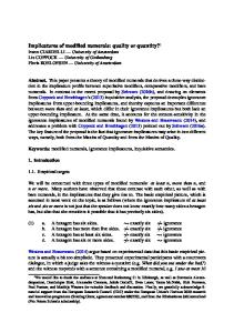
where C is a positive constant. As a consequence, the low Mach asymptotics of the linear wave Equation (1.14) is simply given by Pq 0 (x). Figure 1.1 represents schematically the solution of the linear wave equation.

1.1.3

The low Mach asymptotics in the case of the perturbed linear wave equation

The key points to obtain (1.15) are that E = KerL and that (1.14) conserves the energy. In fact, we can relax these two properties in the following way: Theorem 1.1.2. Let L be a linear operator and let q(t, x) be solution of the linear equation   ∂ q + L q = 0, t M  q(t = 0) = q 0

(1.16)

13

1.1. THE LOW MACH NUMBER PROBLEM

Figure 1.1: Solution q of the linear wave Equation (1.14). The incompressible component of the solution is Pq 0 ∈ E and its acoustic component is q − Pq ∈ E⊥ . e 0 || for any t ≥ 0, where C e is a positive supposed to be well-posed in such a way that ||q||(t) ≤ C||q constant (which in particular does not depend on M ). We recall that the subspace E is invariant for (1.16) if q 0 (·) ∈ E =⇒ ∀t ≥ 0, q(t, ·) ∈ E (see (7)) where q is the solution of (1.16). Moreover, we recall that P is the orthogonal projection on E. Let C be another positive constant. Then: 1) When E is invariant for (1.16), we have ||q 0 − Pq 0 || = CM 2) When L is such that

=⇒

e ∀t ≥ 0, ||q − Pq||(t) ≤ C CM.

E ⊆ KerL,

(1.17)

(1.18)

we have ||q 0 − Pq 0 || = CM

=⇒

e ∀t ≥ 0, ||q − Pq 0 ||(t) ≤ C CM.

(1.19)

This result is useful to have a first understanding of the low Mach number problem. Indeed, let us consider that L := L + δL where δL is a perturbation (which may depend on M ) deduced from the truncation error of a given numerical scheme applied to (1.14) on a cartesian mesh. Estimate (1.17) means that Equation (1.16) does not create any acoustic waves of order one in the acoustic subspace E⊥ when ||q 0 − Pq 0 || = O(M ) although the discretization introduces an error through δL. Estimate (1.19) characterizes the fact that the solution q(t, x) of (1.16) remains close at any time to the low Mach asymptotics Pq 0 of the linear wave equation (1.14) when ||q 0 −Pq 0 || = O(M ) although the discretization introduces an error through the perturbation δL in L. Proof of Theorem 1.1.2: The proof of Point 1 is written in [11] (see Point 2 of Theorem 2.2 in [11]). Nevertheless, since the proof of Point 2 follows the steps of the proof of Point 1, we reproduce it here for the sake of convenience. Point 1: Let us define qe(t, x) and q(t, x) solutions of (1.16) with the respective initial conditions qe0 = Pq 0 and q 0 = q 0 − Pq 0 . By linearity, we have q = qe + q. Moreover ||q − Pq|| = ||e q − Pe q + q − Pq|| = ||q − Pq|| since E is invariant for (1.16). Then, we have ||q − Pq|| ≤ ||q||

(1.20)

14CHAPTER 1. THE LOW MACH NUMBER PROBLEM ANALYZED WITH THE LINEAR WAVE EQUATIO e 0 || and ||q 0 || = since (1 − P) is an orthogonal projection. On the other hand, we have ||q|| ≤ C||q ||q 0 − Pq 0 || = CM . Thus, we have e ||q|| ≤ C CM (1.21) e by using (1.20). which allows to obtain ||q − Pq|| ≤ C CM Point 2: Under Condition (1.18), we have qe = Pq 0 . Thus, we have q − Pq 0 = q which allows to e by using (1.21). obtain ||q − Pq 0 || ≤ C CM

1.1.4

A first definition of an accurate scheme at low Mach number

Estimate (1.19) suggests to write that the solution q(t, x) of (1.16) is accurate at low Mach number in the incompressible regime of the linear wave equation if and only if the estimate + 0 0 0 ∀C1 ∈ R+ ∗ , ∃C2 ∈ R∗ such that ||q − Pq || = C1 M =⇒ ∀t ≥ 0, ||q − Pq ||(t) ≤ C2 M

(1.22)

is satisfied, C2 being a positive parameter that depends on C1 and that does not depend on M . In this definition, the ”incompressible regime” means that we consider initial data that are close to the incompressible space E. Point 2 of Theorem 1.1.2 means that a sufficient condition to be accurate at low Mach number in the sense of (1.22) is that E ⊆ KerL. Let us underline that when E 6⊆ KerL, we cannot tell whether the solution q(t, x) is or is not accurate at low Mach number in the sense of (1.22) since (1.18) is only a sufficient condition. In that case, we have to carefully study the time behaviour of (1.16) to verify if Estimate (1.22) is or is not satisfied. In the same way, Estimate (1.17) leads us to say that the solution q(t, x) of (1.16) is free of any spurious acoustic wave if and only if the estimate + 0 0 ∀C1 ∈ R+ ∗ , ∃C2 ∈ R∗ such that ||q − Pq || = C1 M =⇒ ∀t ≥ 0, ||q − Pq||(t) ≤ C2 M

(1.23)

is satisfied. Of course, (1.22) is stronger than (1.23) since for any q and q 0 , we have ||q−Pq|| ≤ ||q−Pq 0 ||. Point 1 of Theorem 1.1.2 underlines that the invariance of E in the energy space (L2 (T))1+d is a sufficient condition to avoid spurious acoustic waves in the sense of (1.23). Nevertheless, the invariance of E is not sufficient to be accurate at low Mach number in the sense of (1.22). Estimates (1.22) and (1.23) are useful to analyze the accuracy of a given scheme at low Mach number and, in particular, to propose a low Mach correction for low Mach flows, as we will see it in §1.1.5 and §1.1.6 in the case of Godunov type schemes. Nevertheless, we will also see in §1.2 that in the case of Godunov type schemes, we will have to relax (1.22) and (1.23) in order to propose and to justify an all Mach Godunov type scheme.

1.1.5

A first explanation of the right or wrong behaviour of Godunov type schemes at low Mach number through the study of discrete kernels

We show in this section that the low Mach number problem can be analyzed as we analyzed in §1.1.3 the low Mach asymptotics in the linear perturbed case (1.16). For that purpose, let us suppose that the domain Ω included in Rd (d ∈ {1, 2, 3}) is discretized by N cells Ωi . Let Γij be the common edge or face of two neighboring cells Ωi and Ωj and nij be the unit vector normal to Γij pointing from Ωi to Ωj . The semi-discrete Godunov scheme applied to the resolution of the linear wave equation (1.14) is given by  X d a∗ 1    ri + · |Γij | [(ui + uj ) · nij + ri − rj ] = 0, (1.24a)   M 2|Ωi |  dt Γij ⊂∂Ωi

d a∗ 1    ui + ·   dt M 2|Ω i| 

X Γij ⊂∂Ωi

|Γij | [ri + rj + κ(ui − uj ) · nij ] nij = 0

(1.24b)

15

1.1. THE LOW MACH NUMBER PROBLEM

with κ = 1. We introduce the parameter κ in (1.24b) for reasons that will appear in the sequel (let us note that (1.24) is the Godunov scheme if and only if κ = 1). This scheme can be written in the compact form   d q + Lκ,h q = 0, ri h h dt M with qh := (1.25) ui  0 qh (t = 0) = qh where the subscript h recalls that (1.25) comes from a spatial discretization of (1.14) (h is a characteristic length of the mesh). The kernel KerLκ,h of the discrete acoustic operator Lκ,h is given by   X ri KerLκ,h := ∈ RN (1+d) such that |Γij | [(ui + uj ) · nij + ri − rj ] = 0,  ui Γij ⊂∂Ωi   X and |Γij | [ri + rj + κ(ui − uj ) · nij ] nij = 0 . (1.26)  Γij ⊂∂Ωi

We have the following result: Lemma 1.1.2. rh KerLκ=1,h = qh := ∈ RN (1+d) uh

such that

∃a ∈ R, ∀i : ri = c

and

(ui − uj ) · nij = 0 (1.27)

and KerLκ=0,h

rh ∈ RN (1+d) = qh := uh

such that

∃a ∈ R, ∀i : ri = c X

and

Γij ⊂∂Ωi

  ui + uj |Γij | · nij = 0 .  2

(1.28)

Moreover, we have KerLκ=1,h ⊆ KerLκ=0,h .

(1.29)

By using Point 2 of Theorem 1.1.2 with Lemma 1.1.2, we obtain a first explanation of the right or wrong behaviour of Godunov type schemes at low Mach number in 1D, 2D and 3D for different type of meshes. Indeed, Lemma 1.1.2 shows that KerLκ=1,h – which is the kernel in the case of the Godunov scheme – may not be a good approximation of E because the continuity of u · n on each edge Γij of the mesh could be too restrictive for particular meshes (e.g. when the mesh is cartesian). On the other hand, Lemma 1.1.2 shows also that KerLκ=0,h may be a good approximation of E for any mesh type because Z X ui + uj |Γij | · nij ' ∇ · u dx. (1.30) 2 Ωi Γij ⊂∂Ωi

Thus, by also using (1.29), we can say that at the discrete level, KerLκ=1,h may not satisfy (1.18) and that KerLκ=0,h may satisfy (1.18). These points are studied in [15] when the mesh is cartesian or triangular, and it is shown that (see Lemmas 5.1, 5.2 and 5.6 in [15]):     on a 2D triangular mesh:

on a 1D cartesian mesh:    on a 2D or 3D cartesian mesh:

KerLκ=1,h = E∆ h ⊂ KerLκ=0,h , KerLκ=1,h = KerLκ=1,h

E h = KerLκ=0,h , E h = KerLκ=0,h

(1.31a) (1.31b) (1.31c)

16CHAPTER 1. THE LOW MACH NUMBER PROBLEM ANALYZED WITH THE LINEAR WAVE EQUATIO where E∆ hoc approximations of E which depend on the type of mesh. We recall the h and Eh are ad ⊥ ⊥ ∆ ∆ definitions of Eh , Eh , Eh and E in Annex A. In (1.31b) and (1.31c), we suppose that the h number of cells is odd in each direction. If it is not the case, we have to replace (1.31b) and (1.31c) by  KerLκ=1,h = E  on a 1D cartesian mesh: h ⊂ KerLκ=0,h ,



on a 2D or 3D cartesian mesh: KerLκ=1,h

E h ⊂ KerLκ=0,h

because of the existence of checkerboard modes in the kernel KerLκ=0,h . By using these relations between the discrete kernels and the discrete incompressible spaces, and by using the sufficient condition (1.18), we can say that in the sense of Definition (1.22):  on a 2D triangular mesh: the Godunov scheme (i.e. (1.24) with κ = 1) is accurate at low Mach     number,    on a 1D cartesian mesh: the Godunov scheme (i.e. (1.24) with κ = 1) is accurate at low Mach number,      on a 2D or 3D cartesian mesh: the modified Godunov scheme obtained with (1.24) and κ = 0 is accurate   at low Mach number. This leads us to define in §1.1.6 the low Mach Godunov type scheme with (1.24) and κ = 0. On the other hand, we cannot conclude from (1.31c) anything about the accuracy on a 2D or 3D cartesian mesh of the Godunov scheme (i.e. (1.24) with κ = 1) in the sense of Definition (1.22) since (1.18) is only a sufficient condition. However, by studying the short time behaviour of (1.24) when κ = 1, we proved in [15] (see §5.3.2 in [15]) that On a 2D or 3D cartesian mesh, the Godunov scheme (i.e. (1.24) with κ = 1) is not accurate at low Mach number. Proof of Lemma 1.1.2: The proof uses the fact that for any qh ∈ KerLκ,h defined by (1.26), we have h i X |Γij | (ri − rj )2 + κ [(ui − uj ) · nij ]2 = 0. (1.32) Γij

This relation was proven in [15] (see (88) in [15]). As a consequence, when κ = 1, we obtain that ∀i : ri = c and (ui − uj ) · nij = 0. Let us now suppose that κ = 0. Thus, when qh ∈ KerLκ=0,h X , we only deduce from (1.32) that ∀i : ri = c. And, by injecting ri = c in (1.26), we find |Γij |(ui + uj ) · nij = 0. The converse is obtained by using the fact that Γij ⊂∂Ωi

X Γij ⊂∂Ωi

|Γij |nij = 0

(1.33)

and X Γij ⊂∂Ωi

|Γij |ui · nij = ui ·

X Γij ⊂∂Ωi

|Γij |nij = 0

(1.34)

We obtain (1.29) by using again (1.33) and (1.34).

1.1.6

A low Mach Godunov type scheme in the linear and non-linear case

This approach leads us to modify the Godunov scheme by replacing κ = 1 in (1.24) with κ = 0 to recover the accuracy at low Mach number. This corresponds to centering the discretization of ∇r in the acoustic operator. The non-linear version of the linear scheme (1.24) with κ = 0, applied to the compressible Euler system (1) or to the barotropic Euler system (2), consists in modifying any X scheme of Godunov type (e.g. X = Roe [36] or X = VFRoe [5]) in such a way that the discretization of the pressure gradient ∇p is centered. We named this class of schemes low Mach X schemes in [11]. Low Mach number numerical test cases validate this approach in [11].

17

1.1. THE LOW MACH NUMBER PROBLEM

1.1.7

Numerical results in the linear case with an initial condition q 0 ∈ E

We illustrate the influence of the cell geometry on the Godunov scheme applied to the linear wave equation (see Equation (1.31) of §1.1.5). We consider the 2D domain Ω = [0, 1]2 with periodic boundary conditions. The initial conditions q 0 := (r0 , u0 )T are given by  r(t = 0, x, y) = 1,    ux (t = 0, x, y) = sin2 (πx) sin(2πy), (1.35)    uy (t = 0, x, y) = − sin(2πx) sin2 (πy) which is periodic on the torus [0, 1]2 . Thus, we have q 0 ∈ E (that is to say q 0 = Pq 0 ) which implies that q = q0 (1.36) is solution of the linear wave equation (1.14). From a numerical point of view, we use periodic boundary 4 0 conditions and we project q 0 on E h (resp. Eh ), which provides the numerical initial condition qh : thus, 4 by construction, we have qh0 = Ph qh0 where Ph is the discrete Hodge projection on E h (resp. Eh ). We −4 −3 choose a∗ = 1, M = 10 and the final time is t = 10 × M = 10 . In Figure 1.2, we show that (1.36) is satisfied at the discrete level when we solve the linear wave equation (1.14) with the linear Godunov scheme (1.24) on a triangular mesh. In Figure 1.3, we show that (1.36) is not satisfied with the linear Godunov scheme on a cartesian mesh since the solution is extremely diffused over time. On cartesian meshes, we need to correct the linear Godunov scheme. If we use the linear low Mach Godunov scheme of §1.1.6 on cartesian meshes, Figure 1.4 shows that (1.36) is satisfied again. From a theoretical point of view, all these results are explained by the study of the discrete kernel of the spatial operator associated to the linear Godunov scheme (see (1.31)).

Triangular mesh

Legend

Initial time

Final time: Godunov scheme

Figure 1.2: Velocity magnitude kuk obtained at initial time t = 0 and at final time t = 10−3 = 10 × M with the linear Godunov scheme on a triangular mesh (700 cells) for an initial incompressible −4 state q 0 ∈ E4 h and a Mach number M = 10 . According to Equation (1.31a), the initial incompressible state q 0 ∈ E4 h is preserved over time with the linear Godunov scheme on a triangular mesh.

1.1.8

Toward an all Mach Godunov type scheme in the non-linear case

In the sequel of this paper, we modify the non-linear low Mach X scheme defined in §1.1.6 in such a way that it is identical to the X scheme when the Mach number is greater than one. In other words, we introduce all Mach Godunov type schemes which are expected to be stable and accurate on both rectangular and triangular meshes and for any Mach number. For that purpose, we clearly define in §1.2 what ”accurate” means in the linear case. Then, we construct in §1.3 the all Mach Godunov type schemes still in the linear case, and we extend it to the non-linear barotropic case in §2.1 and to the fully compressible case in §3.1.

18CHAPTER 1. THE LOW MACH NUMBER PROBLEM ANALYZED WITH THE LINEAR WAVE EQUATIO

Cartesian mesh

Legend

Initial time

Final time: Godunov scheme

Figure 1.3: Velocity magnitude kuk obtained at initial time t = 0 and at final time t = 10−3 = 10 × M with the linear Godunov scheme on a cartesian mesh (30 × 30 cells with ∆x = ∆y = 0.33) for an −4 initial incompressible state q 0 ∈ E h and a Mach number M = 10 . According to Equation (1.31c), 0 the initial condition q ∈ Eh is not preserved over time with the linear Godunov scheme on a cartesian mesh. The solution is extremely diffused over time.

Cartesian mesh

Legend

Initial time

Final time: low Mach Godunov scheme

Figure 1.4: Velocity magnitude kuk obtained at initial time t = 0 and at final time t = 10−3 = 10 × M with the linear low Mach Godunov scheme on a cartesian mesh (30×30 cells with ∆x = ∆y = 0.33) for −4 an initial condition q 0 ∈ E h and a Mach number M = 10 . According to Equation (1.31c), the initial 0 condition q ∈ Eh is preserved over time with the linear low Mach Godunov scheme on a cartesian mesh. The linear low Mach Godunov scheme allows to preserve q 0 ∈ E h on cartesian meshes.

1.2. DEFINITION OF AN ACCURATE SCHEME AT LOW MACH NUMBER IN THE LINEAR CASE19

1.2

Definition of an accurate scheme at low Mach number in the linear case

Estimate (1.22) is suggested by Estimate (1.15) of Corollary 1.1.1 which concerns the linearization (1.8) of the barotropic Euler System (1.5) with H := 0. But, when H 6= 0, Estimate (1.15) cannot be satisfied by the solution q(t, x) of (1.8) and has to be replaced by Estimate (1.12) of Proposition 1.1.1. Nevertheless, we have the following result: Lemma 1.2.1. Let q(t, x) be solution of   ∂ q + Hq + L q = 0, t M  q(t = 0, x) = q 0 (x)

(1.37)

with q 0 ∈ L2 (T) × (C 1 (T))d . Then, we have ∀(C1 , C2 ) ∈ R+ ∗

2

0 0 , ∃C3 ∈ R+ ∗ such that ||q − Pq || = C1 M

=⇒ ∀t ∈ [0, C2 M ], ||q − Pq 0 ||(t) ≤ C3 M,

(1.38)

C3 being a positive parameter that depends on (C1 , C2 ) and that does not depend on M . As a consequence, the important point is to verify if Estimate (1.22) is or is not satisfied only for short times. Thus, we relax (1.22) and we propose the following definition: Definition 1. The solution q(t, x) of   ∂ q + L q = 0, t M  q(t = 0) = q 0

(1.39)

is said to be accurate at low Mach number for short times in the incompressible regime of the linear wave equation if and only if the estimate ∀(C1 , C2 ) ∈ R+ ∗

2

0 0 , ∃C3 ∈ R+ ∗ such that ||q − Pq || = C1 M

=⇒ ∀t ∈ [0, C2 M ], ||q − Pq 0 ||(t) ≤ C3 M

(1.40)

is satisfied, C3 being a positive parameter that depends on (C1 , C2 ) and that does not depend on M . A second reason that justifies the study of ||q − Pq 0 ||(t) for short times and not for long times is that the boundary conditions may have an important influence on the behaviour of ||q − Pq 0 ||(t) for long times. For example, ||q − Pq 0 ||(t) may be small for short times and large for long times with periodic boundary conditions although ||q − Pq 0 ||(t) could remain small for any time with transparent boundary conditions when it is small for short times. Let us recall that we impose in this paper periodic boundary conditions. Thus, we will construct in the sequel a numerical scheme for which the solution of the associated first order modified equation is accurate at low Mach number in the sense of (1.40) but not in the sense of (1.22). Let us note that we can keep (1.23) for the spurious acoustic waves when H 6= 0 because of Estimate (1.13) of Proposition 1.1.1. Nevertheless, when a solution q(t, x) is accurate at low Mach number in the sense of Definition 1, we are sure that this solution is free of any spurious acoustic wave in short time (this is a consequence of the fact that for any q and q 0 , we have ||q − Pq|| ≤ ||q − Pq 0 ||); but we can say nothing a priori in long time. Thus, we also relax (1.23) with:

20CHAPTER 1. THE LOW MACH NUMBER PROBLEM ANALYZED WITH THE LINEAR WAVE EQUATIO

Fig. 1.5(a) (1.40) and (1.42) are verified

Fig. 1.5(b) (1.40) is not verified, (1.42) is verified

Fig. 1.5(c) (1.40) and (1.42) are not verified

Figure 1.5: Explanation of the low Mach problem: different behaviours based on Definitions 1 and 2. Definition 2. The solution q(t, x) of   ∂ q + L q = 0, t M  q(t = 0) = q 0

(1.41)

is said to be free of any spurious acoustic wave for short times if and only if the estimate ∀(C1 , C2 ) ∈ R+ ∗

2

0 0 , ∃C3 ∈ R+ ∗ such that ||q − Pq || = C1 M =⇒ ∀t ∈ [0, C2 M ], ||q − Pq||(t) ≤ C3 M

(1.42)

is satisfied, C3 being a positive parameter that depends on (C1 , C2 ) and that does not depend on M . Figure 1.5 describes three different behaviours based on Definitions 1 and 2: Figure 1.5(a) describes a solution q(t, x) which is accurate at low Mach number; Figure 1.5(b) describes a solution q(t, x) which is not accurate at low Mach number but which is free of any spurious acoustic wave; Figure 1.5(c) describes a solution q(t, x) which is not accurate at low Mach number and which is not free of spurious acoustic waves. The numerical results proposed in §1.3.3 will be coherent with Figure 1.5. Proof of Lemma 1.2.1: We have ||q − Pq 0 ||(t) ≤ q − Tu∗ ,t Pq 0 (t) + Tu∗ ,t Pq 0 − Pq 0 (t) where Tu∗ ,t is the application defined by (Tu∗ ,t f )(x) = f (x − u∗ t). Thus, by using (1.12), we obtain that ||q 0 − Pq 0 || = C1 M =⇒ ∀t ≥ 0 : ||q − Pq 0 ||(t) ≤ C1 M + Tu∗ ,t Pq 0 − Pq 0 (t). On the other hand, for any q := (r, u)T ∈ E, we have (since r is a constant in space): Z 2 ||Tu∗ ,t q − q|| (t) = |u(x − u∗ t) − u(x)|2 dx. T

d But, for any u ∈ C 1 (T) , we have |u(x − u∗ t) − u(x)| ≤ |u∗ |t max |∇u| T

2

with |∇u| :=

d X k=1

|∇uk |2 where u := (u1 , . . . , ud )T , d is the spatial dimension and | · | is the euclidian

norm in Rd . Thus ∀t ∈ [0, C2 M ] : ||Tu∗ ,t q − q|| (t) ≤ C2 M |u∗ | max |∇u| · |T| T

1.3. CONSTRUCTION AND JUSTIFICATION OF AN ALL MACH GODUNOV SCHEME IN THE LINEAR CA with |T| :=

R

T dx.

This allows to write that ∀t ∈ [0, C2 M ] : Tu∗ ,t Pq 0 − Pq 0 (t) ≤ C2 M |u∗ | max |∇u0 | · |T| T

where Pq 0 = (r0 , u0 )T , which gives the result with C3 = C1 + C2 |u∗ | max |∇u0 | · |T|. T

1.3

Construction and justification of an all Mach Godunov scheme in the linear case

In this section, we construct a modified Godunov type scheme which is asymptotically identical to the linear low Mach Godunov scheme (see (1.24) with κ = 0) when M 1 and which is identical to the linear Godunov scheme (see (1.24) with κ = 1) when M = O(1). We justify this construction by using the tools introduced in §1.1. We name this linear scheme all Mach Godunov scheme. The non-linear versions of this linear all Mach Godunov scheme will be directly obtained in §2.1 and §3.1 from the linear approach proposed below.

1.3.1

The case of the linear wave equation on a cartesian mesh

This subsection is devoted to the cartesian case. This case is interesting because it allows to propose an all Mach Godunov type scheme through a simple study of the first order modified equation associated with the Godunov scheme (1.24)κ=1 applied to the linear wave equation (1.14). Let us define the 2D system   ∂ q + Lν q = 0, t M  q(t = 0, x) = q 0 (x)

(1.43)

with x := (x, y), q := (r, u)T , u := (ux , uy )T and  Lν = L − M B ν

   with Bν q =   

νr ∆r ∂ 2 ux νux ∂x2 ∂ 2 uy νuy ∂y 2

      

(1.44)

where ν := (νr , νu ) ∈ (R+ )3

and

νu := (νux , νuy ) ∈ (R+ )2 .

Thus, (1.43) is a perturbed wave equation whose perturbation is given by δLν = −M Bν . In the 2D cartesian case (the 3D cartesian case is similar) [11], the first order modified equation of the Godunov scheme (1.24)κ=1 applied to the linear wave equation (1.14) is given by (1.43)(1.44) with ν = ν G where ν G := (νrG , νuG )

and

νrG := a∗

∆x , 2M

νuG := a∗

∆x (1, 1) 2M

(∆x is the mesh size supposed to be identical in the directions x and y for the sake of simplicity). We prove that (see Lemma 4.3 in [11]): Lemma 1.3.1. 1) In 1D with νr ≥ 0, νux ≥ 0:

KerLν = E.

22CHAPTER 1. THE LOW MACH NUMBER PROBLEM ANALYZED WITH THE LINEAR WAVE EQUATIO 2) In 2D with νr ≥ 0, νux = νuy = 0:

KerLν = E.

3) In 2D with νr ≥ 0, νux > 0 and νuy > 0: r KerLν = q := ∈ (L2 (T))3 such that u

∃c ∈ R : r = c

and

∂x ux = ∂y uy = 0

E. (1.45)

The extension of Lemma 1.3.1 to the 3D case is straightforward. We deduce from Point 2 of Theorem 1.1.2 and from Point 3 of Lemma 1.3.1 that the solution q(t, x) of (1.43)(1.44) may not be accurate at low Mach number in the incompressible regime as soon as the spatial dimension is 2D (or 3D) and νu is not equal to zero. Indeed, in that case, we do not have E ⊆ KerLν (see (1.18)). However, the situation is more involved since E ⊆ KerLν is only a sufficient condition: as a consequence, the knowledge of KerLν is not sufficient to have a correct understanding of the low Mach behaviour of the Godunov scheme and of any modified Godunov scheme obtained by modifying the numerical viscosity ν G . Moreover, for a particular choice of νu , we may expect that the short time estimate (1.40) is satisfied even if the long time estimate (1.22) is not satisfied. In that case, the solution q(t, x) would be accurate at low Mach number in the sense of Definition 1. This is illustrated by the following result: Theorem 1.3.1. Let q(t, x) be the solution of the 2D equation (1.43)(1.44). Then, for any νr ≥ 0: 1) When νu = νuG , for almost all function q 0 ∈ (L2 (T))3 , q(t, x) verifies ∀C1 ∈ R+ ∗,

∃(C2 , C3 ) :

||q 0 − Pq 0 || = C1 M

=⇒

∀t ≥ C2 M, ||q − Pq 0 ||(t) ≥ C3 ∆x

(1.46)

C3 ∆x, C2 and C3 being positive parameters that respectively depend on T and (T, q 0 ), C1 and that do not depend on M and ∆x. as soon as M ≤

2) When νu = νuG and ∆x = C0 M , for any q 0 ∈ (H 2 (T))3 , q(t, x) verifies 3 ∀(C0 , C1 , C2 ) ∈ R+ , ∃C3 : ||q 0 − Pq 0 || = C1 M =⇒ ∀t ∈ [0, C2 M ], ||q − Pq 0 ||(t) ≤ C3 M, ∗

(1.47) C3 being a positive parameter that depends on (T, q 0 , C0 , C1 , C2 ) and that does not depend on M . Moreover, C3 goes to C1 when C0 goes to zero. 3) When νu = M νuG , for any q 0 ∈ (H 2 (T))3 , q(t, x) verifies 2 ∀(C1 , C2 ) ∈ R+ , ∃C3 : ||q 0 − Pq 0 || = C1 M =⇒ ∗ C3 being a positive parameter that depends on

∀t ∈ [0, C2 M ], ||q − Pq 0 ||(t) ≤ C3 M,

(T, q 0 , C1 , C2 , ∆x)

(1.48) and that does not depend on M .

Again, we easily extend this result to the 3D case. This result shows that the short time behaviours of (1.43)(1.44) with ν = (νr , νuG ) and with ν = (νr , M νuG ) are different although the kernels of L(νr ,νuG ) and of L(νr ,M νuG ) are identical (see Point 3 of Lemma 1.3.1). This is an illustration of the fact that Condition (1.18) is only a sufficient condition to be accurate at low Mach number in the sense of Definition 1. More precisely:

1.3. CONSTRUCTION AND JUSTIFICATION OF AN ALL MACH GODUNOV SCHEME IN THE LINEAR CA • Point 1 of Theorem 1.3.1 and its 3D version show that when the mesh is cartesian, for almost all q 0 ∈ (L2 (T))1+d , the Godunov scheme in 2D/3D is not accurate at low Mach number in the sense of Definition 1 when M ∆x. Let us note that we do not prove that the solution q(t, x) of (1.43)(1.44) is not accurate at low Mach number by producing in short time spurious acoustic waves (see Definition 2 for the notion of spurious acoustic wave). In other words, we prove that the short time behaviour of q(t, x) is characterized by Figure 1.5(b) but we do not prove that it is characterized by Figure 1.5(c). Numerical results proposed in §1.3.3 show that there exist initial conditions q 0 such that spurious acoustic waves are not created in short time – which corresponds to Figure 1.5(b) – and such that spurious acoustic waves are created in short time – which corresponds to Figure 1.5(c).

• Point 2 of Theorem 1.3.1 and its 3D version show that when the mesh is cartesian, for any q 0 ∈ (H 2 (T))1+d , the Godunov scheme in 2D/3D is accurate at low Mach number in the sense of Definition 1 when ∆x = O(M ) or when ∆x M , which is too expensive from a computational point of view.

• Point 3 of Theorem 1.3.1 and its 3D version show that when the mesh is cartesian, for any q 0 ∈ (H 2 (T))1+d , the modified Godunov scheme obtained by replacing νuG with M νuG is accurate at low Mach number in the sense of Definition 1 even when M ∆x. Thus, this scheme is also free of any spurious acoustic waves in the sense of Definition 2. This result is central in our way to construct an all Mach Godunov scheme. At last, we underline that all the results proposed in Theorem 1.3.1 are valid as soon as νr ≥ 0, that is to say not only when νr = νrG . Proof of Theorem 1.3.1: Let q1 (t) be the solution of   ∂ q + Lν q = 0, t 1 1 M  q1 (t = 0, x) = (q 0 − Pq 0 )(x)

(1.49)

and q2 (t) be the solution of   ∂ q + Lν q = 0, 2 t 2 M  q2 (t = 0, x) = Pq 0 (x)

(1.50)

where Lν is defined with (1.44). By linearity, the solution q(t, x) of (1.43)(1.44) satisfies q(t, x) = q1 (t, x) + q2 (t, x). Since ||q − Pq 0 ||(t) = ||q1 + q2 − Pq 0 ||(t), we have ∀t ≥ 0 :

||q − Pq 0 ||(t) ≥ ||q2 − Pq 0 ||(t) − ||q1 ||(t)

(1.51)

∀t ≥ 0 :

||q − Pq 0 ||(t) ≤ ||q1 ||(t) + ||q2 − Pq 0 ||(t).

(1.52)

and Moreover, since (1.49) is a dissipative equation when νr ≥ 0, νux ≥ 0 and νuy ≥ 0 (see Lemma 4.1 in [11]), we obtain ||q1 ||(t) ≤ ||q 0 − Pq 0 || which implies that ∀t ≥ 0 :

||q1 ||(t) ≤ C1 M

(1.53)

since ||q 0 −Pq 0 || = C1 M . We will use below (1.51), (1.52) and (1.53) to prove (1.46), (1.47) and (1.48).

24CHAPTER 1. THE LOW MACH NUMBER PROBLEM ANALYZED WITH THE LINEAR WAVE EQUATIO Proof of Point 1: Let us define the orthogonal projection Pν on KerLν (Pν = P if and only if νr ≥ 0 and νux = νuy = 0; in particular, Pν 6= P when ν = ν G ). In [15], we prove that ∀t ≥

M LT : a∗

||q2 − Pq 0 ||(t) ≥

∆x ||Pq 0 − Pν Pq 0 || 3LT

where LT is a constant which only depends on T (see Estimate (50) of Corollary 4.1 in [15]). Hence ∀t ≥ C2 M :

||q2 − Pq 0 ||(t) ≥ C∆x

(1.54)

LT ||Pq 0 − Pν Pq 0 || and C = . In the sequel, we suppose that C is non-zero, which is the a∗ 3LT case for almost all function q 0 ∈ (L2 (T))3 . Using (1.51), (1.53) and (1.54), we obtain

with C2 =

∀t ≥ C2 M :

||q − Pq 0 ||(t) ≥ C∆x − C1 M.

(1.55)

Let us now consider any M such that C1 M ≤ C3 ∆x

with

C3 =

C . 2

(1.56)

We deduce from (1.55) and (1.56) that ∀t ≥ C2 M : for any M ≤

C3 C1 ∆x,

||q − Pq 0 ||(t) ≥ C3 ∆x

which allows to obtain (1.46).

Proof of Points 2 and 3: Since LP = 0, we deduce from (1.50) that ∂t (q2 − Pq 0 ) +

L (q2 − Pq 0 ) = Bν (q2 − Pq 0 ) + Bν Pq 0 . M

(1.57)

Then, by multiplying (1.57) with q2 − Pq 0 and by integrating, we obtain 1 d · ||q2 − Pq 0 ||2 (t) = hq2 − Pq 0 , Bν (q2 − Pq 0 )i + hq2 − Pq 0 , Bν Pq 0 i 2 dt since hq2 − Pq 0 , L(q2 − Pq 0 )i = 0. And since ( hq2 − Pq 0 , Bν (q2 − Pq 0 )i ≤ 0,

hq2 − Pq 0 , Bν Pq 0 i ≤ ||q2 − Pq 0 || · ||Bν Pq 0 ||,

we can write that d ||q2 − Pq 0 ||(t) ≤ ||Bν Pq 0 || ≤ max(|νux |, |νuy |) · ||Pq 0 ||H 2 dt by using the definition of Bν in (1.44), which gives ∀t ∈ [0, C2 M ] :

||q2 − Pq 0 ||(t) ≤ C2 M · max(|νux |, |νuy |) · ||Pq 0 ||H 2

since ||q2 − Pq 0 ||(0) = 0, that is to say ∀t ∈ [0, C2 M ] : by using (1.52) and (1.53).

||q − Pq 0 ||(t) ≤ C1 + C2 max(|νux |, |νuy |) · ||Pq 0 ||H 2 M

(1.58)

1.3. CONSTRUCTION AND JUSTIFICATION OF AN ALL MACH GODUNOV SCHEME IN THE LINEAR CA Let us now suppose that νu = νuG . In that case, we have max(|νux |, |νuy |) =

that (1.58) is given by

∀t ∈ [0, C2 M ] :

||q − Pq 0 ||(t) ≤

a∗ ∆x which implies 2M

C2 a∗ ∆x C1 + ||Pq 0 ||H 2 M 2M

C0 C2 a∗ ||Pq 0 ||H 2 when ∆x = C0 M . 2 We now suppose that νu = M νuG . In that case, (1.58) is given by C2 a∗ ∆x ||Pq 0 ||H 2 M ∀t ∈ [0, C2 M ] : ||q − Pq 0 ||(t) ≤ C1 + 2

which allows to obtain (1.47) with C3 = C1 +

which allows to obtain (1.48) with C3 = C1 +

1.3.2

C2 a∗ ∆x ||Pq 0 ||H 2 . 2

The case of the linear wave equation on any mesh type

In order to recover accuracy at low Mach number, Points 1 and 3 of Theorem 1.3.1 lead us to modify the Godunov scheme (1.24)κ=1 applied to the linear wave equation   ∂ q + L q = 0, t M (1.59)  0 q(t = 0, x) = q (x) by replacing κ = 1 (which is equivalent to νu = νuG ) with κ = M (which is equivalent to νu = M νuG ) in (1.24). Thus, we propose the all Mach Godunov scheme  d X 1 a∗  r + · |Γij | [(ui + uj ) · nij + ri − rj ] = 0,  i   dt M 2|Ωi | Γij ⊂∂Ωi (1.60) X d a∗ 1   u + · |Γ | [r + r + θ(M )(u − u ) · n ] n = 0  i ij i j i j ij ij  dt M 2|Ωi | Γij ⊂∂Ωi

with θ(M ) = min(M, 1)

(1.61)

which also allows to recover the Godunov scheme (1.24)κ=1 when the Mach number is greater than one. The all Mach Godunov scheme (1.60) may be rewritten as X 1 d r + |Γij |ΦAM,Godunov =0 ij dt u i |Ωi |

(1.62)

Γij ⊂∂Ωi

with the two following expressions for the numerical flux ΦAM,Godunov which are equivalent in this ij linear case1 : • First expression: ΦAM,Godunov ij

=

ΦGodunov ij

a∗ + [θ(M ) − 1] 2M

0 [(ui − uj ) · nij ]nij

(1.63)

where ΦGodunov is the unmodified Godunov flux (ΦGodunov is easily deduced from (1.24)κ=1 ) and ij ij where θ(M ) is defined by (1.61). Thus, the simple corrective flux a∗ 0 [θ(M ) − 1] (1.64) [(ui − uj ) · nij ]nij 2M 1

AM,Godunov

The notation AM in Φij

means that this flux defines an All Mach scheme.

26CHAPTER 1. THE LOW MACH NUMBER PROBLEM ANALYZED WITH THE LINEAR WAVE EQUATIO defines an all Mach correction which is equal to zero when the Mach number is greater than one. This all Mach correction introduces numerical anti-diffusion since θ(M ) − 1 ≤ 0. At last, we can note that the linear all Mach Godunov scheme (1.62)(1.63) may be seen as the Godunov scheme plus a pressure a∗ correction since the correction [θ(M ) − 1] [(ui − uj ) · nij ]nij in (1.64) is homogeneous to a pressure. 2M • Second expression: The flux (1.63) is equivalent to ΦAM,Godunov ij

a∗ = M

(u · n)∗ r∗∗ n

! with ij

∗∗ ∗ rij = θ(M )rij + [1 − θ(M )]

ri + rj 2

(1.65)

where (r∗ , (u · n)∗ ) is solution of the 1D linear Riemann problem in the nij direction  Lζ   qζ = 0, ∂t qζ +    M    ri ζ < 0 : qζ (t = 0, ζ) = , ui · nij      rj    ζ ≥ 0 : qζ (t = 0, ζ) = u · n j ij with qζ :=

r uζ

and Lζ qζ := a∗ ∂ζ

uζ r

(1.66)

, ζ being the coordinate in the nij direction. This gives

 ri + rj (ui − uj ) · nij  ∗  = + ,  rij 2 2  (u + uj ) · nij ri − rj   (u · n)∗ij = i + . 2 2 The linear all Mach Godunov scheme (1.62)(1.63) – which is equivalent to (1.62)(1.65)2 – may be seen as a Godunov type scheme whose Riemann solver is corrected to be accurate at low Mach number.

1.3.3

Numerical results on a 2D cartesian mesh

Firstly, we justify the linear all Mach Godunov scheme (1.61)(1.62)(1.63) on cartesian meshes by testing it with the initial condition qh0 ∈ E h used in §1.1.7. The results are presented in Figure 1.6 and can be compared to the one obtained with the linear Godunov scheme (see Figure 1.3) which is defined with (1.62)(1.63) where θ(M ) := 1. Even if qh0 ∈ E h is not exactly preserved over time when we solve the linear wave equation (1.14) with the linear all Mach Godunov scheme on a cartesian mesh (because of (1.31c)), the results are better with the linear all Mach Godunov scheme since the initial condition seems to be preserved over time. Secondly, we justify Points 1 and 3 of Theorem 1.3.1 and the linear all Mach Godunov scheme with numerical results obtained on a 2D cartesian mesh by studying the error kqh − Ph qh0 k(t) obtained with the linear Godunov scheme and with the linear all Mach Godunov scheme. For that purpose, we modify a little bit the initial condition of §1.1.7 by adding an orthogonal component of the order 0 + M q 0 where q 0 ∈ E of M . This means that we can write the initial condition qh0 as qh0 = qh,1 h,2 h,1 h 2

The non-linear versions of (1.62)(1.63) and (1.62)(1.65) are not equivalent: see §2.1 and §3.1.

1.3. CONSTRUCTION AND JUSTIFICATION OF AN ALL MACH GODUNOV SCHEME IN THE LINEAR CA

Cartesian mesh

Legend

Initial time

Final time: all Mach Godunov scheme

Figure 1.6: Velocity magnitude kuk obtained at initial time t = 0 and at final time t = 10−3 = 10 × M with the linear all Mach Godunov scheme on a cartesian mesh (30 × 30 cells with ∆x = ∆y = 0.33) −4 for an initial condition q 0 ∈ E h (see Equation (1.35)) and a Mach number M = 10 . The linear all Mach Godunov scheme gives better results than those obtained with the linear Godunov scheme (see Figure 1.3). 0 ∈ E and qh,2 h

         

⊥

0 k = 1. This initial condition is given by with kqh,2

r(t = 0, x, y) =

1

ux (t = 0, x, y) =

sin2 (πx) sin(2πy)

+ + M

         uy (t = 0, x, y) = − sin(2πx) sin2 (πy) + M

0

,

cos(2πx) cos(2πy) k(0, cos(2πx) cos(2πy), − sin(2πx) sin(2πy))k

,

− sin(2πx) sin(2πy) k(0, cos(2πx) cos(2πy), − sin(2πx) sin(2πy))k

.

(1.67)

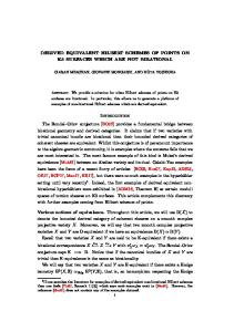
Moreover, we consider a coarse cartesian mesh (30 × 30 cartesian mesh with ∆x = ∆y = 0.033) and a small Mach number M = 10−4 . In Figure 1.7, we plot the error kqh − Ph qh0 k(t) generated with each scheme as a function of time. The linear Godunov scheme is not accurate at low Mach number in the sense of Defintion 1 (see Point 1 of Theorem 1.3.1). Indeed, with the linear Godunov scheme, the norm of the deviation kqh − Pqh0 k(t) is greater than ∆x = ∆y = 0.033 for times of the order of M = 10−4 . However, the linear all Mach Godunov scheme is accurate at low Mach number (see Point 3 of Theorem 1.3.1) since the norm of the deviation kqh − Pqh0 k(t) remains of the order of M for times of the order of M = 10−4 : this is exactly the configuration of Figure 1.5(a). In Figure 1.7, we also represent kqh − Pqh0 k(t) obtained with the linear all Mach Godunov scheme until an asymptotic state is reached. This point justifies Definition 1 which only considers the short time behaviour on which the linear all Mach Godunov scheme is accurate although its long time behaviour is the same as the one of the linear Godunov scheme in a periodic domain. Figure 1.8 represents kqh −Pqh k(t) = kqh⊥ k ⊥ for 0 ≤ t/M ≤ 10 with M = 10−4 where qh⊥ is the projection of qh in (E h ) . Here, the important point is that the Godunov scheme is such that the energy kqh − Pqh k(t) = kqh⊥ k(t) of the acoustic part of the solution remains of the order of M on a time scale of order M although kqh −Pqh0 k(t) is of order one (see Figure 1.7). In this particular case, the Godunov scheme is not accurate at low Mach number in the sense of Definition 1 (see Figure 1.7) but is free of spurious acoustic waves in the sense of Definition 2.

28CHAPTER 1. THE LOW MACH NUMBER PROBLEM ANALYZED WITH THE LINEAR WAVE EQUATIO

0.4

0.00024

0.35

0.00022 0.0002

0.3

0.00018

0.25

∥qh − Pqh0 ∥

∥qh − Pqh0 ∥

AM-Godunov

Godunov AM-Godunov

0.2 0.15

0.00016 0.00014 0.00012

0.1

0.0001

0.05

8e-05 6e-05

0 0

1

2

3

4

5

6

7

8

9

0

10

1

2

3

4

5

6

7

8

9

10

t/M

t/M 0.4

AM-Godunov

0.35

∥qh − Pqh0 ∥

0.3 0.25 0.2 0.15 0.1 0.05 0 0

10000 20000 30000 40000 50000 60000 70000 80000 90000100000 t/M

Figure 1.7: Norm of the deviation kqh − Pqh0 k(t) as a function of time for M = 10−4 (0 ≤ t/M ≤ 10 for 1 the top pictures and 0 ≤ t/M ≤ 105 for the bottom picture) obtained with an1 initial condition q 0 = q10 + ⊥ (see Equation (1.67)) on a 30×30 cartesian mesh. The scales are not the same for all M q20 ∈ E h + Eh figures. The linear Godunov scheme is not accurate at low Mach number (see Point 1 of Theorem 1.3.1) since the norm of the deviation kqh − Pqh0 k(t) (top left picture) is much greater than ∆x = ∆y = 0.033 for times of the order of M = 10−4 . The linear all Mach Godunov scheme is accurate at low Mach number (see Point 3 of Theorem 1.3.1) since the norm of the deviation kqh −Pqh0 k(t) (top right picture) remains of the order of M for times of the order of M = 10−4 : this is exactly the configuration of Figure 1.5(a). The bottom picture represents kqh −Pqh0 k(t) obtained with the linear all Mach Godunov scheme until an asymptotic state is reached. This point justifies Definition 1 which only considers the short time behaviour. Indeed, the long time behaviours of the linear Godunov scheme and of the linear all Mach Godunov scheme are the same in a periodic domain. 1

1.3. CONSTRUCTION AND JUSTIFICATION OF AN ALL MACH GODUNOV SCHEME IN THE LINEAR CA This is exactly the configuration of Figure 1.5(b). This particular result is due to the form of the 0 = Pq 0 of the initial condition (1.67) which satisfies ∂ 0 0 incompressible part qh,1 xxx ux,1 + ∂yyy uy,1 = 0. h Indeed, setting Du := ∂xxx ux + ∂yyy uy , it may be proved by simple algebraic manipulations that when νux = νuy =: ν, the triplet (r, ∇ · u, Du) solves the following equations: a∗ ∇ · u − νr ∆r = 0, M a∗ ∂t (∇ · u) + ∆r − νDu = 0, M a∗ ∂t (Du) + (∂xxxx + ∂yyyy )r + ν∂xxyy (∇ · u) − ν∆(Du) = 0, M

∂t r +

so that when starting from an initial condition such that r0 = 1, ∇ · u0 = 0 and Du0 = 0, the solution (r, u) remains in the incompressible space E. And thus the initial incompressible part of the ⊥. solution q10 does not transfer energy from the incompressible space E h to the acoustic space Eh Let us note that in the case of the initial condition (1.67), we can also verify this result by computing the exact solution u1 (t). Indeed, (1.67) implies that 1 1 sin(2πy) − cos(2πx) sin(2πy), 2 2 1 1 = − sin2 (πy) sin(2πx) = − sin(2πx) + cos(2πy) sin(2πx), 2 2

u01,x = u01,y

sin2 (πx) sin(2πy)

=

and it can be checked that (1, 21 sin(2πy), − 12 sin(2πx))T is in the kernel of the perturbed wave operator, and that (0, − cos(2πx) sin(2πy), cos(2πy) sin(2πx))T is an eigenvector of the perturbed wave operator when νux = νuy =: ν, associated to the eigenvalue 4π 2 ν. Thus, the initial condition (1.67) gives rise to 1 1 sin(2πy) − cos(2πx) sin(2πy) exp(−4π 2 νt), u1,x (t) = 2 2 1 1 u1,y (t) = − sin(2πx) + cos(2πy) sin(2πx) exp(−4π 2 νt). 2 2 As a consequence, the solution is free of spurious acoustic waves in the sense of Definition 2 although it is inaccurate at low Mach number in the sense of Definition 1 when ν = ν G . 0.00011

Godunov AM-Godunov

0.0001 9e-05 ∥qh − Pqh ∥ = ∥qh⊥ ∥

8e-05 7e-05 6e-05 5e-05 4e-05 3e-05 2e-05 1e-05 0 0

1

2

3

4

5

6

7

8

9

10

t/M

Figure 1.8: Norm of the acoustic wave kqh − Pqh k(t) = kqh⊥ k(t) as a function of time for 0 ≤ t/M ≤ 10 ⊥ (see Equation (1.67)) with M = 10−4 obtained with an initial condition q 0 = q10 + M q20 ∈ E h + Eh on a 30 × 30 cartesian mesh (∆x = ∆y = 0.033). The linear Godunov scheme does not produce ⊥ spurious acoustic waves in E since kqh − Pqh k(t) = kqh⊥ k(t) remains of the order of M for times h 0 of order M = 10−4 . This is due to the fact that the initial incompressible part qh,1 = Pqh0 of the 0 0 initial condition satisfies ∂xxx ux,1 + ∂yyy uy,1 = 0. In this particular case, the linear Godunov scheme is not accurate at low Mach number in the sense of Definition 1 (see Figure 1.7) but is free of spurious acoustic waves in the sense of Definition 2: this is exactly the configuration of Figure 1.5(b).

30CHAPTER 1. THE LOW MACH NUMBER PROBLEM ANALYZED WITH THE LINEAR WAVE EQUATIO

To better understand the behaviour of the Godunov scheme and of the all Mach Godunov scheme 0 = Pq 0 of the initial condition (1.67) such in the general case, we modify the incompressible part qh,1 h 0 does not satisfy ∂ 0 0 that qh,1 xxx ux,1 + ∂yyy uy,1 = 0. This new initial condition is given by          

r(t = 0, x, y) =

1

ux (t = 0, x, y) =

2 sin2 (πx) sin(4πy)

+ + M

         uy (t = 0, x, y) = − sin(2πx) sin2 (2πy) + M

0

,

cos(2πx) cos(2πy) k(0, cos(2πx) cos(2πy), − sin(2πx) sin(2πy))k

,

− sin(2πx) sin(2πy) k(0, cos(2πx) cos(2πy), − sin(2πx) sin(2πy))k

.

(1.68)

The conclusion of Figure 1.9 is the same as the one of Figure 1.7: the all Mach Godunov scheme is accurate at low Mach number and the Godunov scheme is not accurate at low Mach number in the sense of Definition 1. However, if we focus on kqh − Pqh k(t) = kqh⊥ k(t) (see Figure 1.10), we see that the energy kqh − Pqh k(t) = kqh⊥ k(t) of the acoustic part of the solution grows up to values of the order of ∆x = 0.033 on a time scale of order M . Thus, by transfering energy from the incompressible ⊥ , the Godunov scheme is no longer free of spurious acoustic waves space E h to the acoustic space Eh ⊥ in E : this is exactly the configuration of Figure 1.5(c). However, the linear all Mach Godunov h scheme is free of spurious acoustic waves in the sense of Definition 2 since kqh − Pqh k(t) = kqh⊥ k(t) remains of the order of M for times of the order of M = 10−4 . Thirdly, we justify Point 2 of Theorem 1.3.1. Figure 1.11 shows that the Godunov scheme is accurate at low Mach number if we take a mesh such that ∆x = ∆y M . For this illustration, we consider a finer cartesian mesh (100 × 100 cartesian mesh with ∆x = ∆y = 0.01) and a larger Mach number M = 10−1 . The norms of the deviations from the initial condition kqh − Pqh0 k(t) obtained with the Godunov scheme and the all Mach Godunov scheme remain of the order of M for times of the order of M = 10−1 . This property is no more satisfied for long times. We note that this computation can be done because the Mach number is not so small (M = 10−1 ). Indeed, the computation cannot be done on a classical computer for a mesh satisfying ∆x = ∆y M if M = 10−4 . This remark also justifies the all Mach Godunov scheme because of the numerical cost of the Godunov scheme on cartesian meshes such that ∆x = ∆y M for small Mach number M .

1.3. CONSTRUCTION AND JUSTIFICATION OF AN ALL MACH GODUNOV SCHEME IN THE LINEAR CA

0.0006

0.6

AM-Godunov

0.00055

0.5

0.0005 0.00045 ∥qh − Pqh0 ∥

∥qh − Pqh0 ∥

0.4 Godunov AM-Godunov

0.3 0.2

0.0004 0.00035 0.0003 0.00025 0.0002 0.00015

0.1

0.0001 5e-05

0 0

1

2

3

4

5

6

7

8

9

0

10

1

2

3

4

5

6

7

8

9

10

t/M

t/M 0.6 0.5

∥qh − Pqh0 ∥

0.4 AM-Godunov

0.3 0.2 0.1 0 0

10000 20000 30000 40000 50000 60000 70000 80000 90000 100000 t/M

Figure 1.9: Norm of the deviation kqh − Pqh0 k(t) as a function of time for M = 10−4 (0 ≤ t/M ≤ 10 for 1 the top pictures and 0 ≤ t/M ≤ 105 for the bottom picture) obtained with an1 initial condition q 0 = q10 + ⊥ (see Equation (1.68)) on a 30×30 cartesian mesh. The scales are not the same for all M q20 ∈ E h + Eh figures. The linear Godunov scheme is not accurate at low Mach number (see Point 1 of Theorem 1.3.1) since the norm of the deviation kqh − Pqh0 k(t) (top left picture) is much greater than ∆x = ∆y = 0.033 for times of the order of M = 10−4 . The linear all Mach Godunov scheme is accurate at low Mach number (see Point 3 of Theorem 1.3.1) since the norm of the deviation kqh −Pqh0 k(t) (top right picture) remains of the order of M for times of the order of M = 10−4 : this is exactly the configuration of Figure 1.5(a). The bottom picture represents kqh −Pqh0 k(t) obtained with the linear all Mach Godunov scheme until an asymptotic state is reached. This point justifies Definition 1 which only considers the short time behaviour. Indeed, the long time behaviours of the linear Godunov scheme and of the linear all Mach Godunov scheme are the same in a periodic domain. 1

32CHAPTER 1. THE LOW MACH NUMBER PROBLEM ANALYZED WITH THE LINEAR WAVE EQUATIO

0.05

0.04

9e-05

0.035

8e-05

0.03 0.025 0.02 0.015

7e-05 6e-05 5e-05 4e-05 3e-05

0.01

2e-05

0.005

1e-05

0 0

1

2

3

4

5

6

7

AM-Godunov

0.0001

∥qh − Pqh ∥ = ∥qh⊥ ∥

∥qh − Pqh ∥ = ∥qh⊥ ∥

0.00011

Godunov AM-Godunov

0.045

8

9

0

10

0

1

2

3

4

t/M

5

6

7

8

9

10

t/M

Figure 1.10: Norm of the spurious acoustic wave kqh − Pqh k(t) = kqh⊥ k(t) as a function of time ⊥ for 0 ≤ t/M ≤ 10 with M = 10−4 obtained with an initial condition q 0 = q10 + M q20 ∈ E + E h h (see Equation (1.68)) on a 30 × 30 cartesian mesh (∆x = ∆y = 0.033). The linear Godunov scheme ⊥ produces spurious acoustic waves in E since the energy kqh − Pqh k(t) = kqh⊥ k(t) of the acoustic h part of the solution grows up to values of the order of ∆x on a time scale of order M : this is exactly the configuration of Figure 1.5(c). The linear all Mach Godunov scheme is free of spurious acoustic waves in the sense of Definition 2 since kqh − Pqh k(t) = kqh⊥ k(t) remains of the order of M for times of order M = 10−4 .

1

1

0.55

Godunov AM-Godunov

0.5 0.45

∥qh − Pqh0 ∥

0.4 0.35 0.3 0.25 0.2 0.15 0.1 0.05 0

2

4

6

8

10

t/M

Figure 1.11: Norm of the deviation kqh −Pqh0 k(t) as a function of time for 0 ≤ t/M ≤ 10 and M = 10−1 ⊥ (see Equation (1.68)) on a 100 × 100 obtained with an initial condition q 0 = q10 + M q20 ∈ E h + Eh cartesian mesh. The Godunov scheme and the all Mach Godunov scheme are accurate at low Mach number on fine cartesian meshes (∆x = ∆y = M/10) (see Point 2 of Theorem 1.3.1). Indeed, the norms of the deviations kqh − Pqh0 k(t) obtained with the Godunov scheme and with the all Mach Godunov scheme remain of the order of M for times of the order M = 10−1 . This property is no more satisfied for long times. Moreover, the all Mach Godunov scheme is more accurate at low Mach number than the Godunov scheme.

1

Chapter 2

The non-linear barotropic case This second chapter can be read without reading Chapter 1. Godunov type schemes are known to be inacurrate at low Mach number (the Mach number will be denoted in what follows by M ): their solutions do not reproduce the correct asymptotic behaviour of flows when M → 0. This is known as, and will be called here, the low Mach number problem. In Chapter 1, we analyzed this issue on the simple linear wave equation   ∂ q + L q = 0, t M (2.1)  0 q(t = 0, x) = q (x) with q = (r, u)T and Lq = a∗ (∇ · u, ∇r)T where a∗ = C st such that O(a∗ ) = 1 (the notation O(f ) means of the order of f ), where u is the flow velocity and r is a rescaled pressure, and we proposed a correction to the Godunov scheme that allows to recover a correct accuracy at low Mach number, while being identical to the standard Godunov scheme for Mach numbers greater than or equal to 1. Indeed, on a mesh with cells denoted by Ωi , interfaces between cells Ωi and Ωj denoted by Γij and unit normal vector from Ωi to Ωj denoted by nij , the standard Godunov scheme for Equation (2.1) can be written as  d X a∗ 1  r + · |Γij | [(ui + uj ) · nij + ri − rj ] = 0,  i   dt M 2|Ωi | Γij ⊂∂Ωi (2.2) X d a∗ 1   u + · |Γ | [r + r + κ(u − u ) · n ] n = 0  i ij i j i j ij ij  dt M 2|Ωi | Γij ⊂∂Ωi

with κ = 1. In this linear case, the proposed correction amounts to replace κ in (2.2) by a function θ(M ) := min(M, 1), so that the corrected scheme is given by X d 1 r + |Γij |ΦAM,Godunov =0 (2.3) ij dt u i |Ωi | Γij ⊂∂Ωi

with the following two expressions for the numerical flux ΦAM,Godunov which are equivalent in the ij 1 linear case : • First expression: ΦAM,Godunov ij

=

ΦGodunov ij

a∗ + [θ(M ) − 1] 2M

0 [(ui − uj ) · nij ]nij

(2.4)

where ΦGodunov is the unmodified Godunov flux (ΦGodunov is easily deduced from (2.2)κ=1 ). Thus, the ij ij simple corrective flux a∗ 0 [θ(M ) − 1] (2.5) [(ui − uj ) · nij ]nij 2M 1

AM,Godunov

The notation AM in Φij

means that this flux defines an All Mach scheme.

33

34

CHAPTER 2. THE NON-LINEAR BAROTROPIC CASE

defines an all Mach correction which is equal to zero when the Mach number is greater than one. This all Mach correction introduces numerical anti-diffusion since θ(M ) − 1 ≤ 0. At last, we can note that the linear all Mach Godunov scheme (2.3)(2.4) may be seen as the Godunov scheme plus a pressure a∗ correction since the correction [θ(M ) − 1] [(ui − uj ) · nij ]nij in (2.5) is homogeneous to a pressure. 2M • Second expression: The flux (2.4) is equivalent to ΦAM,Godunov ij

a∗ = M

(u · n)∗

! with

r∗∗ n

ij

∗∗ ∗ rij = θ(M )rij + [1 − θ(M )]

ri + rj 2

(2.6)

where (r∗ , (u · n)∗ ) is solution of the 1D linear Riemann problem in the nij direction  Lζ   qζ = 0, ∂t qζ +    M    ri ζ < 0 : qζ (t = 0, ζ) = , ui · nij      r j    ζ ≥ 0 : qζ (t = 0, ζ) = u · n j ij with qζ :=

r uζ

and Lζ qζ := a∗ ∂ζ

uζ r

(2.7)

, ζ being the coordinate in the nij direction. This gives

 (ui − uj ) · nij ri + rj  ∗  + , =  rij 2 2  (u + uj ) · nij ri − rj   (u · n)∗ij = i + . 2 2 The aim of Chapter 2 is to extend the all Mach correction defined above to the non-linear barotropic Euler system (2). Chapter 2 is usefull to understand from a practical point of view how to quickly introduce the all Mach correction in a code that solves the non-linear barotropic Euler system with a Godunov type scheme. When the Godunov type scheme is a Roe scheme, we prove that it remains possible to obtain linear stability results when we use an all Mach correction and we justify this correction in the non-linear case with a formal asymptotic analysis. In particular, the link between this formal asymptotic analysis and some results obtained in Chapter 1 in the linear case is detailed. In Chapter 3, we extend and we test with numerous test cases the proposed non-linear all Mach correction to the full compressible Euler system (1). The outline of Chapter 2 is the following. From the linear approach recalled above, we propose all Mach Godunov type schemes in §2.1 in the case of the barotropic Euler system (2). We propose in §2.2 a linear stability result for these non-linear schemes when the Godunov type scheme is a Roe scheme, and we justify in §2.3 the accuracy of this non-linear scheme with a formal asymptotic expansion. §2.2 and §2.3 concern also the all Mach schemes proposed in [34, 31].

2.1

Construction of all Mach Godunov type schemes in the barotropic case

We now extend the linear all Mach Godunov schemes (2.3)(2.4) and (2.3)(2.6) to the non-linear case when the linear wave equation (2.1) is replaced by the barotropic Euler system (2). This leads us to propose the non-linear all Mach Godunov type scheme d dt

ρ ρu

+ i

1 |Ωi |

X Γij ⊂∂Ωi

|Γij |ΦAM,X =0 ij

(2.8)

2.1. CONSTRUCTION OF ALL MACH GODUNOV TYPE SCHEMES IN THE BAROTROPIC CASE35 with again two possible expressions for the numerical flux ΦAM,X . In (2.8), X is a Godunov type ij scheme: e.g. X=Godunov [17], X = Roe [36], X = VFRoe [5] or X = Lagrange + Projection type scheme (see §2.2.5). The two possible expressions for ΦAM,X are the following: ij • First expression: The non-linear version of (2.4) is given by ρij aij 0 AM,X X Φij = Φij + (θij − 1) [(ui − uj ) · nij ] nij 2

(2.9)

where ΦX ij is the unmodified flux given by the X scheme and where θij = θ(Mij )

with

θ(M ) = min(M, 1),

(2.10)

Mij , ρij and aij being estimates at the edge Γij respectively of the Mach number, the density and the sound velocity. Thus, the all Mach correction is now given by ρij aij 0 (2.11) (θij − 1) [(ui − uj ) · nij ] nij 2 and introduces anti-diffusion since θij − 1 ≤ 0. The flux ΦAM,Roe obtained with (2.9) and when X is ij the Roe scheme [36] is specified in Annex C in the subsonic case (see (C.8)). • Second expression: The non-linear version of (2.6) is given by ! ρ∗ (u · n)∗ pi + pj AM,X Φij = with p∗∗ = θij p∗ij + (1 − θij ) ij 2 ρ∗ (u∗ · n)u∗ + p∗∗ n ij

(2.12)

where (ρ∗ , u∗ ) is solution of a 1D (linearized or non-linearized) Riemann problem. Let us note that p∗∗ in (2.12) replaces p∗ := p(ρ∗ ). As in the linear case (see (2.3)(2.6)), the non-linear all Mach X scheme (2.8)(2.12) may be seen as a Godunov type scheme whose Riemann solver is corrected to be accurate at low Mach number. We underline that the non-linear all Mach X schemes (2.8)(2.9) (which is the non-linear version of (2.3)(2.4)) and (2.8)(2.12) (which is the non-linear version of (2.3)(2.6)) are not equivalent although the linear schemes (2.3)(2.4) and (2.3)(2.6) are equivalent. Definition of the Mach number Mij : The Mach number Mij in (2.10) may be defined with Mij := |uij | |uij · nij | or with Mij := (uij and aij are estimates at the edge Γij respectively of the velocity aij aij and the sound velocity), the second one giving a less dissipative scheme (especially for shear flows for which we may have uij ⊥ nij ). Moreover, the linear stability result proposed in Theorem 2.2.1 is valid with these two definitions of the Mach number Mij . Nevertheless, the numerical results proposed in |uij | this paper are obtained by using Mij := to define the all Mach correction (2.11). aij We know that the Godunov scheme applied to the barotropic Euler system (2) is stable (and entropic) for any Mach number and is not always accurate at low Mach number (for example on a two or three-dimensional cartesian mesh). The aim of the all Mach Godunov scheme is to obtain an accurate scheme at low Mach number on any mesh type. However, since in the all Mach Godunov scheme we reduce the numerical diffusion of the Godunov scheme, we are not sure that the all Mach Godunov scheme remains stable for any Mach number. In the following two sections, we partly justify the stability and the accuracy of the all Mach Godunov scheme applied to the barotropic Euler system (2) on any mesh type and for any Mach number. More precisely:

36

CHAPTER 2. THE NON-LINEAR BAROTROPIC CASE • In Section 2.2, we (partly) justify the stability question by proposing a linear stability result in the subsonic case for (2.8)(2.9) when the X scheme is the Roe scheme [36]. • In Section 2.3, we (partly) justify the accuracy question with a formal asymptotic expansion applied to (2.8)(2.9) when the X scheme is the Roe scheme [36].

2.2

A linear stability result in the subsonic barotropic case

We now prove a linear stability result for the all Mach Godunov type schemes (2.8)(2.9). This result (partly) justifies the stability question of the all Mach Godunov type schemes. We study this stability question by extending the linear Godunov scheme (2.3)(2.4) to the linear system   ∂ q + Hq + L q = 0, t M (2.13)  q(t = 0, x) = q 0 (x) where u∗ ∈ Rd (d ∈ {1, 2, 3}) is a constant velocity field such that O(|u∗ |) = 1. Here, it is important to take into account the linear transport operator Hq := (u∗ · ∇)q because the discretization of this operator has an impact on the stability of the all Mach Godunov scheme as we will see below. This is due to the fact that the Godunov approach does not split the material and acoustic waves (respectively L described with ∂t q + Hq = 0 and ∂t q + q = 0). This leads us to conclude this section with a remark M on the Lagrange + Projection approach which splits the material and acoustic waves.

2.2.1

The linear all Mach Godunov scheme in the subsonic case

When the Godunov scheme is applied to System (2.13) and when the flow is subsonic i.e. |u∗ | <

a∗ M

(subsonic condition),

(2.14)

the Godunov flux ΦGodunov is given by (see (B.8) in Annex B) ij ΦGodunov = ΦGodunov,convection + ΦGodunov,acoustic ij ij ij

(2.15)

where ΦGodunov,convection ij

1 = 2

!

(u∗ · nij ) [ri + rj + (ui − uj ) · nij ] (u∗ · nij ) [(ui + uj ) + (ri − rj )nij ] − |u∗ · nij | [(ui − uj ) × nij ] × nij

(2.16) and ΦGodunov,acoustic ij

a∗ = 2M

(ui + uj ) · nij + ri − rj [ri + rj + (ui − uj ) · nij ] nij

! .

(2.17)

Fluxes (2.16) and (2.17) discretize respectively the linear convection operator Hq and the linear L acoustic operator M q. Flux (2.17) is of course identical to the Godunov flux in (2.2). To obtain the all Mach version ΦAM,Godunov of ΦGodunov defined by (2.15), we just add the all Mach corij ij rection (2.5) to ΦGodunov as in (2.4). Thus, this consists in replacing the acoustic flux ΦGodunov,acoustic ij ij defined by (2.17) by the all Mach acoustic flux a∗ 0 Godunov,acoustic ΦAM,Godunov,acoustic = Φ + [θ(M ) − 1] ij ij [(ui − uj ) · nij ] nij 2M

2.2. A LINEAR STABILITY RESULT IN THE SUBSONIC BAROTROPIC CASE

37

|u∗ | |u∗ | M since M ach = < 1, a∗ /M being the sound velocity a∗ a∗ /M in (2.13)2 (we have M ach = O(M ) since O(|u∗ |) = O(a∗ ) = 1). In other words, we do not correct the convective flux ΦGodunov,convection defined by (2.16), which is coherent with the fact that the low ij Mach number problem is only linked to a wrong discretization of the acoustic operator at low Mach number. with θ(M ) := min(M ach, 1) =

To summarize, under the subsonic condition (2.14), the linear all Mach Godunov scheme applied to (2.13) is given by  X  1 d   (2.18a) r + |Γ | (u∗ · nij ) [ri + rj + γ(M )(ui − uj ) · nij ] i ij   2|Ωi |  dt  Γij ⊂∂Ωi   o   a∗   + [(u + u ) · n + r − r ] = 0, i j ij i j   M   X d 1 (2.18b) ui + |Γij | (u∗ · nij ) [(ui + uj ) + ζ(M )(ri − rj )nij ]   dt 2|Ωi |  Γ ⊂∂Ω  ij i      − β(M )|u∗ · nij | [(ui − uj ) × nij ] × nij      a∗   [ri + rj + θ(M )(ui − uj ) · nij ] nij = 0 +  M with (γ, ζ, β)(M ) := (1, 1, 1). The parameters γ(M ), ζ(M ) and β(M ) are introduced in (2.18) to also study below the influence of the consistency error terms (ui − uj ) · nij in (2.18a), (ri − rj )nij |u∗ | a∗ M, 1 , we γ(M )+ζ(M ) ∈ [0, 1] and 2

in (2.18b) and [(ui − uj ) × nij ] × nij in (2.18b) on the stability. When θ(M ) := min

will see below that (2.18) is stable for any γ(M ), ζ(M ) and β(M ) such that β(M ) ≥ 0. This suggests that we can improve the accuracy of the all Mach Godunov scheme with particular choices of γ(M ), ζ(M ) and β(M ): in [34, 31], the authors propose all Mach schemes which |u∗ | are equivalent in the linear case to (2.18) with θ(M ) := min a∗ M, 1 and with particular choices of γ(M ), ζ(M ) and β(M ). At last, it is important to underline that, as long as γ(M ), ζ(M ) and β(M ) remain of the order of a constant independent of the Mach number M , they have no influence on the M −1 term of the asymptotic expansion of 2.18 when M → 0, and thus have no influence on the low Mach number problem as defined in the introduction of this Chapter 2: only the parameter θ(M ) has an influence on the low Mach number problem (see §2.3).

2.2.2

L2 -stability in the semi-discrete subsonic case

Let us define the energy Eh =

X i

|Ωi | ri2 + |ui |2 .

We have the following L2 -stability result (we recall that since a∗ /M defined the sound velocity in (2.13)):

|u∗ | a∗ M

below is equal to the Mach number

Theorem 2.2.1. Let (r, u) be solution of (2.18). Under the subsonic condition (2.14), for any γ(M ), ) ζ(M ) and β(M ) such that γ(M )+ζ(M ∈ [0, 1] and β(M ) ≥ 0: 2 1) When θ(M ) := 1, we have: d Eh ≤ 0. (2.19) dt Thus, in particular, the Godunov scheme (obtained also with γ(M ) = ζ(M ) = β(M ) = 1) satisfies (2.19). 2

The quantity a∗ /M is the sound velocity in (2.13) because M is such that

p p0 (ρ)/M is the sound velocity in (1.4).

38

CHAPTER 2. THE NON-LINEAR BAROTROPIC CASE

2) When θ(M ) := min

|u∗ | M, 1 , we have: a∗ d Eh ≤ 0. dt

(2.20)

Thus, in particular, the all Mach Godunov scheme (obtained also with γ(M ) = ζ(M ) = β(M ) = 1) satisfies (2.20). 3) When θ(M ) := 0, we have: d γ(M ) + ζ(M ) X Eh ≤ |Γij | |u∗ · nij | |(ui − uj ) · nij |2 . dt 2

(2.21)

Γij

Thus, in particular, the low Mach Godunov scheme (obtained also with γ(M ) = ζ(M ) = β(M ) = 1) satisfies (2.21). The three points of Theorem 2.2.1 are illustrated with numerical results in §2.2.3. Let us note that |u∗ · n| |u∗ | Point 2 of Theorem 2.2.1 is also satisfied with θ(M ) := M instead of θ(M ) := M. a∗ a∗ Discussion about Theorem 2.2.1: Inequality (2.19) confirms that the Godunov scheme is stable. Inequality (2.20) shows that the all Mach Godunov scheme is stable and, thus, justifies from the stability point of view the all Mach correction (2.11). Moreover, inequalities (2.19) and (2.20) with (γ, ζ, β) 6= (1, 1, 1) suggest that we can also improve the accuracy of the Godunov scheme and of the all Mach Godunov scheme by choosing for example γ(M ) = |u∗ | ζ(M ) = β(M ) = min a∗ M, 1 : in [34], Rieper proposes an all Mach scheme that corresponds to the choices ζ(M ) = β(M ) = 1 and γ(M ) = θ(M ) := min |ua∗∗ | M, 1 ; in [31], Oßwald et al. propose an all Mach scheme that corresponds to the choices ζ(M ) = 1 and γ(M ) = β(M ) = θ(M ) := min |ua∗∗ | M, 1 . Of course, other choices are possible: for example γ(M ) = ζ(M ) = β(M ) = θ(M ) := min |ua∗∗ | M, 1 or γ(M ) = −ζ(M ) = β(M ) = θ(M ) := min |ua∗∗ | M, 1 . d ) Inequality (2.21) prevents from obtaining Eh ≤ 0 when u∗ 6= 0 and γ(M )+ζ(M 6= 0. As a conse2 dt quence, we may observe numerical instabilities with the low Mach Godunov scheme when u∗ 6= 0 and γ(M )+ζ(M ) 6= 0. Nevertheless, when u∗ := 0 – i.e. when we restrict the stability analysis to the low 2 Mach Godunov scheme applied to the linear wave equation (i.e. to scheme (2.2) with κ = 0) –, the low Mach Godunov scheme is stable. On the other hand, inequality (2.21) suggests also that we can choose θ(M ) = 0 from the stability point of view when we choose ζ(M ) = −γ(M ). In §2.2.3, we will study the scheme obtained with ζ(M ) = β(M ) = −γ(M ) = 1 and θ(M ) = 0 (together with the all Mach Godunov scheme, the scheme of Rieper [34] and the scheme of Oßwald et al. [31]). Proof of Theorem 2.2.1: Before proving Points 1, 2 and 3, we perform some preliminary calculations. Preliminary calculations: By multiplying (2.18a) by 2|Ωi |ri and by summing with respect to i, we obtain X X d X |Ωi |ri2 = − |Γij | [(u∗ · nij ) [ri + rj + γ(M )(ui − uj ) · nij ] ri dt i i Γij ⊂∂Ωi i a∗ + [(ui + uj ) · nij + ri − rj ] ri . (2.22) M

2.2. A LINEAR STABILITY RESULT IN THE SUBSONIC BAROTROPIC CASE

39

On the other hand, by using X Γij ⊂∂Ωi

|Γij |nij = 0,

we obtain

(2.23)

 X X

|Γij |(u∗ · nij )ri2 =

Γij ⊂∂Ωi

i

X i



ri2 u∗ ·

X Γij ⊂∂Ωi

|Γij |nij  = 0.

Moreover X X Γij ⊂∂Ωi

i

X

|Γij |(u∗ · nij )ri rj =

Γij

|Γij | [u∗ · (nij + nji )] ri rj = 0

since nij + nji = 0. We deduce from the last two equalities that X X i

Γij ⊂∂Ωi

|Γij |(u∗ · nij )(ri + rj )ri = 0.

(2.24)

We have also X X X X |Γij |(u∗ ·nji ) [(uj − ui ) · nji ] rj |Γij |(u∗ ·nij ) [(ui − uj ) · nij ] ri + |Γij |(u∗ ·nij ) [(ui − uj ) · nij ] ri = i

Γij ⊂∂Ωi

Γij

Γij

which gives X X i

Γij ⊂∂Ωi

|Γij |(u∗ · nij ) [(ui − uj ) · nij ] ri =

Moreover

X Γij

|Γij |(u∗ · nij ) [(ui − uj ) · nij ] (ri − rj ).

(2.25)

a∗ X X a∗ X X |Γij | [(ui + uj ) · nij ] ri = |Γij |(uj · nij )ri M M Γij ⊂∂Ωi

i

i

Γij ⊂∂Ωi

by using again (2.23). We have also that a∗ X X a∗ X |Γij | [ri uj · nij + rj ui · nji ] , |Γij |(uj · nij )ri = M M i

Γij ⊂∂Ωi

Γij

which allows to write a∗ X X a∗ X |Γij | [(ui + uj ) · nij ] ri = |Γij | [ri uj − rj ui ] · nij . M M i

Γij ⊂∂Ωi

(2.26)

Γij

At last, we have a∗ X X a∗ X a∗ X |Γij |(ri − rj )ri = |Γij |(ri − rj )ri + |Γij |(rj − ri )rj . M M M i

Γij ⊂∂Ωi

Hence

Γij

Γij

a∗ X X a∗ X |Γij |(ri − rj )ri = |Γij | · |ri − rj |2 . M M i

Γij ⊂∂Ωi

(2.27)

Γij

Thus, by using (2.22), (2.24), (2.25), (2.26) and (2.27), we find X d X 2 |Ωi |ri = − |Γij | γ(M )(u∗ · nij ) [(ui − uj ) · nij ] (ri − rj ) dt i

Γij

+

i a∗ (ri uj − rj ui ) · nij + |ri − rj |2 . (2.28) M

40

CHAPTER 2. THE NON-LINEAR BAROTROPIC CASE

Let us now multiply (2.18b) by 2|Ωi |ui . By summing with respect to i and using the fact that for any vector w there holds that (w × n) · u = −w · (u × n), we obtain X X d X 2 |Ωi | |ui | = − |Γij | (u∗ · nij ) [(ui + uj ) + ζ(M )(ri − rj )nij ] · ui dt i i Γij ⊂∂Ωi i a∗ + β(M )|u∗ · nij | [(ui − uj ) × nij ] · (ui × nij ) + [ri + rj + θ(M )(ui − uj ) · nij ] (nij · ui ) . (2.29) M On the other hand, by using the arguments used to obtain (2.24) and (2.26), we respectively find X X i

and

Γij ⊂∂Ωi

|Γij |(u∗ · nij )(ui + uj ) · ui = 0

(2.30)

a∗ X X a∗ X |Γij |(ri + rj )(nij · ui ) = |Γij |(rj ui − ri uj ) · nij . M M i

Γij ⊂∂Ωi

(2.31)

Γij

We have also X X X X |Γij |(u∗ ·nij )(ri −rj )(nij ·ui ) = |Γij |(u∗ ·nij )(ri −rj )(nij ·ui )+ |Γij |(u∗ ·nji )(rj −ri )(nji ·uj ) Γij ⊂∂Ωi

i

Γij

Γij

which allows to write X X X |Γij |(u∗ · nij )(ri − rj )(nij · ui ) = |Γij |(u∗ · nij ) [(ui − uj ) · nij ] (ri − rj ). i

Γij ⊂∂Ωi

(2.32)

Γij

Moreover a∗ X a∗ X X |Γij | [(ui − uj ) · nij ] (nij · ui ) = |Γij | [(ui − uj ) · nij ] (nij · ui ) M M i Γij ⊂∂Ωi Γij a∗ X + |Γij | [(uj − ui ) · nji ] (nji · uj ) M Γij

and therefore a∗ X X a∗ X |Γij | [(ui − uj ) · nij ] (nij · ui ) = |Γij | |(ui − uj ) · nij |2 . M M i

Γij ⊂∂Ωi

(2.33)

Γij

At last, we obtain X X i

Γij ⊂∂Ωi

|Γij | |u∗ · nij | [(ui − uj ) × nij ] · (ui × nij ) =

X Γij

|Γij | |u∗ · nij | |(ui − uj ) × nij |2 . (2.34)

Thus, by using (2.29), (2.30), (2.31), (2.32), (2.33) and (2.34), we find X d X |Ωi | |ui |2 = − |Γij | dt i

Γij

ζ(M )(u∗ · nij ) [(ui − uj ) · nij ] (ri − rj )

io a∗ h (rj ui − ri uj ) · nij + θ(M ) |(ui − uj ) · nij |2 . (2.35) M Finally, by summing (2.28) and (2.35), we obtain +β(M ) |u∗ · nij | |(ui − uj ) × nij |2 +

X d Eh = − |Γij | {[γ(M ) + ζ(M )](u∗ · nij ) [(ui − uj ) · nij ] (ri − rj ) dt Γij io a∗ h +β(M )|u∗ · nij | |(ui − uj ) × nij |2 + |ri − rj |2 + θ(M ) |(ui − uj ) · nij |2 . (2.36) M

41

2.2. A LINEAR STABILITY RESULT IN THE SUBSONIC BAROTROPIC CASE Moreover, we have −2(u∗ · nij ) [(ui − uj ) · nij ] (ri − rj ) ≤ |u∗ · nij | |(ui − uj ) · nij |2 + |ri − rj |2 .

(2.37)

Thus, by using the subsonic condition (2.14) and since |u∗ · nij | ≤ |u∗ |, we obtain −2(u∗ · nij ) [(ui − uj ) · nij ] (ri − rj ) ≤ |u∗ · nij | |(ui − uj ) · nij |2 +

a∗ |ri − rj |2 . M

(2.38)

By using (2.36), this allows to write X γ(M ) + ζ(M ) d 2 2 Eh ≤ − |Γij | |u∗ · nij | β(M ) |(ui − uj ) × nij | − |(ui − uj ) · nij | dt 2 Γij γ(M ) + ζ(M ) a∗ a∗ 2 2 |ri − rj | + θ(M ) |(ui − uj ) · nij | + 1 − M 2 M that is to say X d Eh ≤ − |Γij | dt Γij

a∗ γ(M ) + ζ(M ) θ(M ) − |u∗ · nij | |(ui − uj ) · nij |2 M 2 γ(M ) + ζ(M ) a∗ + 1− |ri − rj |2 (2.39) 2 M

for any β(M ) ≥ 0. Proof of Points 1 and 2: Let us suppose that θ(M ) := 1 (cf. Point 1). Since |u∗ · nij | ≤ |u∗ |, we obd ) tain Eh ≤ 0 when γ(M )+ζ(M ∈ [0, 1] by using the subsonic condition (2.14) and the inequality (2.39). 2 dt |u∗ | When θ(M ) := M (cf. Point 2), we deduce from (2.39) that a∗ X γ(M ) + ζ(M ) γ(M ) + ζ(M ) a∗ d 2 2 Eh ≤ − |Γij | |u∗ | − |u∗ · nij | |(ui − uj ) · nij | + 1 − |ri − rj | dt 2 2 M Γij

which also gives

d Eh ≤ 0 when dt

γ(M )+ζ(M ) 2

Proof of Point 3: When θ(M ) := 0 and

∈ [0, 1].

γ(M )+ζ(M ) 2

∈ [0, 1], we deduce from (2.39) that

d γ(M ) + ζ(M ) X Eh ≤ |Γij | |u∗ · nij | |(ui − uj ) · nij |2 . dt 2 Γij

2.2.3

Numerical results on the L2 -stability in the linear subsonic case

We illustrate Points 1, 2 and 3 of Theorem 2.2.1 with numerical results obtained on a 2D cartesian mesh. For that purpose, we consider the following problem, which was also considered in the numerical results of Chapter 1 for the simple linear wave equation: We consider the 2D domain Ω = [0, 1]2 with periodic boundary conditions. The initial conditions q 0 := (r0 , u0 )T are given by  r(t = 0, x, y) = 1,    ux (t = 0, x, y) = sin2 (πx) sin(2πy), (2.40)    uy (t = 0, x, y) = − sin(2πx) sin2 (πy) which is periodic on the torus [0, 1]2 and belongs to the kernel of the simple linear wave equation (2.13 with u∗ = 0). We study in Figure 2.1 the energy Eh (t) of the numerical solutions obtained from the linear scheme (2.18) approaching the solution of (2.13) for various values of the set (γ(M ), ζ(M ), β(M ), θ(M )):

42

CHAPTER 2. THE NON-LINEAR BAROTROPIC CASE • the linear Godunov scheme (i.e. γ(M ) = ζ(M ) = β(M ) = θ(M ) = 1), • the linear all Mach Godunov scheme (i.e. γ(M ) = ζ(M ) = β(M ) = 1 and θ(M ) := min

|u∗ | a∗ M, 1

• the linear low Mach Godunov scheme (i.e. γ(M ) = ζ(M ) = β(M ) = 1 and θ(M ) = 0) • the all Mach scheme of Rieper [34] (ζ(M ) = β(M ) = 1 and γ(M ) = θ(M ) := min |ua∗∗ | M, 1 ), • the all Mach scheme of Oßwald et al. min |ua∗∗ | M, 1 ),

[31] (ζ(M ) = 1 and γ(M ) = β(M ) = θ(M ) :=

• an hybrid all Mach scheme (obtained with ζ(M ) = β(M ) = −γ(M ) = 1 and θ(M ) = 0). In the numerical results of Chapter 1, the convective part was not taken into account. In other words, (2.13) was solved with (2.18) by choosing u∗ = 0. Now, we choose u∗ = (1, 0)T in (2.13) |u∗ | and (2.18). The parameter M is fixed to 0.5 and a∗ = 1. In that case, the Mach number a∗ /M is equal to M and the subsonic condition (2.14) is satisfied. Let us note that for the scheme of Rieper and for the scheme of Oßwald et al., we have γ(M ) = min |ua∗∗ | M, 1 and ζ(M ) = 1. Thus, thestability condition min

|u∗ | M,1 a∗

γ(M )+ζ(M ) 2

+1

∈ [0, 1] of Theorem 2.2.1 is satisfied for these two schemes since

) ≤ 1. Of course, the stability condition γ(M )+ζ(M ∈ [0, 1] is also satisfied by the low 2 Mach Godunov scheme, the all Mach Godunov scheme and the hybrid all Mach scheme. 2

Figure 2.1 shows that the energy Eh (t) decreases with time with the Godunov scheme, with the all Mach Godunov scheme, with the scheme of Rieper, with the scheme of Oßwald et al. and with the hybrid scheme, which is coherent with Points 1, 2 and 3 of Theorem 2.2.1. Moreover, the low Mach Godunov scheme is not stable since Eh (t) explodes with time, which is coherent with Point 3 of Theorem 2.2.1. We can also remark that the scheme of Oßwald et al. is less dissipative than the scheme of Rieper: this point is mentioned in [31]. Nevertheless, the scheme of Oßwald et al. is more dissipative than the hybrid scheme which is the least dissipative scheme. These last two remarks are also coherent with Point 3 of Theorem 2.2.1. At last, let us note that the results obtained with the all Mach Godunov scheme and with the scheme of Rieper are similar. This can be explained by noting that the decreasing of the energy differs between these two schemes only through the quantity X Γij

|Γij |γ(M )(u∗ · nij ) [(ui − uj ) · nij ] (ri − rj )

(see (2.36)) – which is the discrete version of γ(M ) (∆x u∗,x h∂x r, ∂x ux i + ∆y u∗,y h∂y r, ∂y uy i) (see (2.47) below) –, by noting that γ(M ) = 1 for the all Mach Godunov scheme and that γ(M ) = |u∗ | 1 min a∗ M, 1 = 2 for the scheme of Rieper (since, in the present case, |u∗ | = a∗ = 1 and M = 12 ) and also by noting that ri (t) is close to a constant (equal to 1 in the present case: see (2.40)) for any i and any t ≥ 0 since this is initially the case.

2.2.4

L2 -stability in the continuous subsonic case

To get a better understanding of the importance of the convection operator in Theorem 2.2.1, it is interesting to study the L2 -stability of the 1st order modified equation associated with (2.18) when the

),

43

2.2. A LINEAR STABILITY RESULT IN THE SUBSONIC BAROTROPIC CASE 5.5

4.5 4

Godunov AM-Godunov Rieper Oßwald et al. θ = 0, ζ = β = −γ = 1

1.35 Eh = ∥r2 + |u|2 ∥ℓ1

5

Eh = ∥r2 + |u|2 ∥ℓ1

1.4

Godunov AM-Godunov LM-Godunov Rieper Oßwald et al. θ = 0, ζ = β = −γ = 1

3.5 3 2.5

1.3 1.25 1.2

2

1.15 1.5 1

1.1 0

0.5

1

1.5

2

2.5

3

3.5

0

1

2

3

4

t/M

5

6

7

8

9

10

t/M

Figure 2.1: Linear L2 -stability study: norm of the energy Eh (t) as a function of time for 0 ≤ t/M ≤ 10 and M = 0.5 obtained with the initial condition (2.40) which belongs to the kernel of the linear wave equation (Equation (2.13) with u∗ = 0) on a 30 × 30 cartesian mesh. The energy Eh (t) decreases with time with the Godunov scheme, with the all Mach Godunov scheme, with the scheme of Rieper [34] (whose results are similar to those obtained with the all Mach Godunov scheme), with the scheme of Oßwald et al. [31] and with the hybrid scheme obtained with ζ(M ) = β(M ) = −γ(M ) = 1 and θ(M ) = 0. However, the low Mach Godunov scheme is not stable since the energy Eh (t) explodes with time. Moreover, the hybrid scheme is the least dissipative scheme. These numerical results are coherent with Points 1, 2 and 3 of Theorem 2.2.1. mesh is cartesian. When we suppose for the sake of simplicity that the dimension is 2D, this equation is given by  1 1  ∂ q + Hq + LM q = 0, t M (2.41)  q(t = 0, x) = q 0 (x) where, in the 2D case, H is the perturbed convection operator defined by  Hq = Hq −

2 u + γ(M )u ∆y∂ 2 u γ(M )u∗,x ∆x∂xx x ∗,y yy y



 1 2 r + β(M )|u |∆y∂ 2 u   ζ(M )u∗,x ∆x∂xx ∗,y yy x   2 2 u + ζ(M )u ∆y∂ 2 r β(M )|u∗,x |∆x∂xx y ∗,y yy

(2.42)

and where LM is the perturbed linear acoustic operator defined by  LM q = Lq −

a∗   2 

2 r + ∆y∂ 2 r ∆x∂xx yy 2 u θ(M )∆x∂xx x 2 u θ(M )∆y∂yy y

  . 

(2.43)

By defining the energy with E := hq, qi =

Z Td

(r2 + |u|2 )dx,

we obtain the following result which is the continuous version of Theorem 2.2.1: Theorem 2.2.2. Let q(t, x) be solution of (2.41). Under the subsonic condition (2.14), for any γ(M ), ) ζ(M ) and β(M ) such that γ(M )+ζ(M ∈ [0, 1] and β(M ) ≥ 0: 2 1) When θ(M ) := 1: d E ≤ 0. dt

(2.44)

44

CHAPTER 2. THE NON-LINEAR BAROTROPIC CASE

2) When θ(M ) := min

|u∗ | M, 1 : a∗ d E ≤ 0. dt

(2.45)

γ(M ) + ζ(M ) d E≤ ∆x|u∗,x | · ||∂x ux ||2 + ∆y|u∗,y | · ||∂y uy ||2 . dt 2

(2.46)

3) When θ(M ) := 0:

Proof of Theorem 2.2.2: The proof is similar to the proof of Theorem 2.2.1. Nevertheless, it is more simple since the operators are continuous. Preliminary calculations: By multiplying (2.41) with q and by integrating over Ω, we obtain that d E = − {[γ(M ) + ζ(M )] (∆x u∗,x h∂x r, ∂x ux i + ∆y u∗,y h∂y r, ∂y uy i) dt + β(M ) ∆y|u∗,y | · ||∂y ux ||2 + ∆x|u∗,x | · ||∂x uy ||2 o a∗ ∆x||∂x r||2 + ∆y||∂y r||2 + θ(M ) ∆x||∂x ux ||2 + ∆y||∂y uy ||2 (2.47) + M which is the continuous version of (2.36). Moreover, we have −2∆x u∗,x h∂x r, ∂x ux i ≤ ∆x|u∗,x | ||∂x ux ||2 + ||∂x r||2

which is the continuous version of (2.37). Thus, under the subsonic condition (2.14), we can write that a∗ −2∆x u∗,x h∂x r, ∂x ux i ≤ ∆x|u∗,x | · ||∂x ux ||2 + ∆x ||∂x r||2 M which is the continuous version of (2.38). In the same way, we have −2∆y u∗,y h∂y r, ∂y uy i ≤ ∆y|u∗,y | · ||∂y uy ||2 + ∆y

a∗ ||∂y r||2 . M

Then, we deduce from (2.47) that a∗ γ(M ) + ζ(M ) a∗ γ(M ) + ζ(M ) d 2 E ≤ − ∆x θ(M ) − |u∗,x | ||∂x ux || + ∆y θ(M ) − |u∗,y | ||∂y uy ||2 dt M 2 M 2 γ(M ) + ζ(M ) a∗ + 1− ∆x||∂x r||2 + ∆y||∂y r||2 2 M for any β(M ) ≥ 0, which is the continuous version of (2.39). Proof of Points 1, 2 and 3: We conclude the proof as in the semi-discrete case (see the proof of Theorem 2.2.1).

2.2.5

A remark on the Lagrange + Projection approach

The potential loss of stability when θ(M ) := 0 (see Point 3 of Theorems 2.2.1 and 2.2.2) is directly linked to   2 u + u ∆y∂ 2 u u∗,x ∆x∂xx x ∗,y yy y  1 2 r  u∗,x ∆x∂xx E(q) := −    2 2 u∗,y ∆y∂yy r in (2.42) which is the non-dissipative part of the truncation error of the Godunov scheme applied to the linear equation (2.13). The existence of this non-dissipative truncation error is a consequence of the fact that the Godunov scheme is built by taking into account at the same time the convective and

2.3. FORMAL ASYMPTOTIC ANALYSIS IN THE BAROTROPIC CASE

45

acoustic waves (see Annex B). This suggests that a Lagrange + Projection approach – which consists in splitting the acoustic and convective waves – may not have any stability problem when θ(M ) := 0. Indeed, a Lagrange + Projection approach applied to the linear equation (2.13) consists, at any time step n, in computing an estimate of the solution by solving   ∂ q L + L q L = 0, t M (Lagrange step) (2.48)  L q (t = n∆t, x) = q n (x) and, then, to correct this estimate by solving ( ∂t q + Hq = 0, q(t = n∆t, x) = q L ((n + 1)∆t, x) .

(Projection step)

(2.49)

Let us now suppose that we solve (2.48) with the all Mach Godunov scheme (2.3)(2.4) and that we solve (2.49) with the Godunov scheme (i.e. with the classical upwind scheme). For this particular Lagrange + Projection scheme, the 1st order modified equation is given by   ∂ q + Hq + LM q = 0, t M (2.50)  0 q(t = 0, x) = q (x) where, in the 2D case, H is the perturbed convective operator  2 r + |u |∆y∂ 2 r |u∗,x |∆x∂xx x ∗,y yy  1 2 2 Hq = Hq −  |u∗,x |∆x∂xx ux + |u∗,y |∆y∂yy ux 2 2 u + |u |∆y∂ 2 u |u∗,x |∆x∂xx y ∗,y yy y

   

(2.51)

and where LM is the perturbed linear acoustic operator defined by (2.43). In that case, we easily obtain: Theorem 2.2.3. Let q(t, x) be solution of (2.50). For any θ(M ) ≥ 0, we have: d E ≤ 0. dt It would be also easy to obtain the semi-discrete version of Theorem 2.2.3. Point 3 of Theorem 2.2.2 and Theorem 2.2.3 underline the fact that if the low Mach correction (i.e. θ(M ) := 0) is identical for any Godunov type schemes, the stability analysis of the low Mach scheme obtained with the low Mach correction strongly depends on the type of Godunov type scheme. On the other hand, Point 2 of Theorem 2.2.2 suggests that the all Mach correction is better than the low Mach correction from a stability point of view, which is coherent since the all Mach correction is less anti-dissipative than the low Mach correction.

2.3

Formal asymptotic analysis in the barotropic case

We now (partly) justify the accuracy question with a formal asymptotic analysis applied to the all Mach Godunov type scheme (2.8)(2.9) when X is the Roe scheme [36]. This analysis is classical [21, 35, 34]. The original point in the following calculus is that we clearly link this formal asymptotic analysis to the point of view proposed in Chapter 1. Moreover, we introduce the parameters γ(M ), ζ(M ) and β(M ) already introduced in the linear scheme (2.18) to show that these parameters do not have any influence on the low Mach number problem when |γ(M )|, |ζ(M )| and β(M ) ≥ 0 are lower than a positive constant independent of the Mach number M , these parameters having only an influence on

46

CHAPTER 2. THE NON-LINEAR BAROTROPIC CASE

the stability of the scheme (see Section 2.2). This will allow us to also justify the all Mach schemes proposed in [34, 31] from the low Mach number problem point of view, the all Mach schemes proposed in [34, 31] being similar to (2.8)(2.9) when X is the Roe scheme. When the X scheme is the Roe scheme [36], the dimensionless all Mach Roe scheme deduced from (2.8)(2.9) and restricted to the subsonic case is given by (see (C.9) in Annex C)  X ρij 1 d    ρi + (2.52a) (uij · nij )(ui − uj ) · nij |Γij | (ρi ui + ρj uj ) · nij + γ(M )M   dt 2|Ωi | aij   Γ ⊂∂Ω ij i   i  aij    (ρ − ρ ) =0 + i j   M    X    d (ρi ui ) + 1 |Γij | ρi (ui · nij )ui + ρj (uj · nij )uj (2.52b)   2|Ωi |   dt Γij ⊂∂Ωi

aij (ρi − ρj ) [uij + (uij · nij )nij ] M − β(M )ρij |uij · nij | [(ui − uj ) × nij ] × nij ρij (uij · nij ) + γ(M )M [(ui − uj ) · nij ] uij aij θij 1 + (pi + pj ) + ρij aij (ui − uj ) · nij nij = 0 M2 M +ζ(M )

                        

with γ(M ) = ζ(M ) = β(M ) = 1, pk = p(ρk ), a2ij = θij = θ(Mij )

pi − pj if ρi 6= ρj and a2ij = p0 (ρi ) otherwise, and ρi − ρj

with

θ(Mij ) = min(Mij , 1).

In (2.53), the local Mach number Mij is given by Mij = M

(2.53)

|uij | . Thus, we can write that Mij = O(M ) aij

which means that

θij ≤C (2.54) M where C is a constant of order one (since Mij 1). The parameters γ(M ), ζ(M ) and β(M ) are introduced in (2.52) to also study the all Mach schemes proposed in [34, 31] which are equivalent to (2.52)(2.53) but with (γ, ζ, β)(M ) 6= (1, 1, 1) (see Discussion about Theorem 2.2.1 in §2.2.1 and the numerical results in §2.2.3). We recall that for stability reasons, γ(M ), ζ(M ) and β(M ) are such that γ(M ) + ζ(M ) ∈ [0, 1] 2

and β(M ) ≥ 0

(see Theorems 2.2.1 and 2.2.2). Moreover, we now suppose that e>0 ∃C

such that

∀M > 0 :

e max[|γ(M )|, |ζ(M )|, β(M )] ≤ C.

(2.55)

At last, we impose periodic boundary conditions. Let us now assume the asymptotic expansion for φ = (ρ, u) φ = φ(0) + M φ(1) + M φ(2) + . . . .

(2.56) We remark that since p = p(ρ), there holds that p(0) = p ρ(0) and p(1) = p0 ρ(0) ρ(1) . More (0) (0) (1) (1) p −p p −p (0) 2 (0) (0) (0) 2 (0) over, aij = i(0) j(0) if ρi = 6 ρj and aij = i(1) j(1) = p0 ρi otherwise. Under the ρi −ρj

ρi −ρj

(sufficient) condition (2.55), by plugging (2.56) in (2.52) and by separating the orders M −1 and M 0 , we obtain:

47

2.3. FORMAL ASYMPTOTIC ANALYSIS IN THE BAROTROPIC CASE • Order M −1 : We deduce from (2.52a) that X (0) (0) (0) = 0. |Γij |aij ρi − ρj Γij ⊂∂Ωi

Thus, we have

(0)

X

ρi

Γij ⊂∂Ωi

i

X Γij (0)

X

(0)

|Γij |aij

(0)

(0)

ρi − ρj

= 0 which gives

h i (0) (0) (0) (0) (0) (0) (0) (0) |Γij | aij ρi − ρj ρi + aji ρj − ρi ρj = 0

(2.57)

(0)

with aji = aij . Then, we obtain X Γij

|Γij |aij

∀i :

ρi

(0)

(0) 2

(0)

ρj − ρi

=0

which implies that (0)

= ρ(0) (t)

(2.58) 1/2 (0) (0) (0) because for all i and j, aij > 0. Thus, pi = p(0) (t) and aij = a(0) (t) = p0 ρ0 (t) . Moreover, if |ζ(M )| is of order one, we deduce from (2.52b) and (2.54) that h i X (1) (1) (0) (0) (0) |Γij | pi + pj nij + ζ(M )aij ρi − ρj (uij + (uij · nij )nij ) = 0 Γij ⊂∂Ωi

which gives X Γij ⊂∂Ωi

(1) (1) |Γij | pi + pj nij = 0

(2.59)

by using (2.58). If |ζ(M )| is of order M α with α > 0, we directly deduce (2.59) from (2.52b) and (2.54). Let us note that Equation (2.59) is equivalent to h i X (1) (1) (0) (0) |Γij | pi + pj + κρ(0) a(0) (ui − uj ) · nij nij = 0 (2.60) Γij ⊂∂Ωi

with κ = 0 for the all Mach Roe scheme. Note that we obtain the same relation (2.60) with κ = 0 for the all Mach schemes of Rieper [34] and Oßwald et al. [31]. In the case of the Roe scheme – which is defined by (2.52) and θij = 1 instead of (2.53) –, we obtain (2.60) with κ = 1. • Order M 0 : We deduce from (2.52a) and (2.58) that 1 d (0) ρ (t) + dt 2|Ωi |

X Γij ⊂∂Ωi

h i (0) (0) (1) (1) |Γij | ρ(0) ui + uj · nij + a(0) ρi − ρj = 0.

(2.61)

On the other hand, we have h i X X X (0) (0) (0) (0) (0) (0) |Γij |ρ(0) ui + uj ·nij = ρ(0) |Γij | ui + uj · nij + uj + ui · nji = 0 i

Γij ⊂∂Ωi

Γij

and X X i

Γij ⊂∂Ωi

X h i (1) (1) (1) (1) (1) (1) |Γij |a(0) ρi − ρj = |Γij | a(0) ρi − ρj + a(0) ρj − ρi = 0. Γij

X d d (0) Thus, by using (2.61), we obtain 2|Ωi | ρ (t) = 0 and therefore ρ(0) (t) = 0. In other dt dt i words, we have ∀i :

(0)

ρi

= C st

(2.62)

48

CHAPTER 2. THE NON-LINEAR BAROTROPIC CASE (0)

and, thus, pi

(0)

= C st and aij = C st . By plugging (2.62) in (2.61), we obtain that X Γij ⊂∂Ωi

h i (0) (0) (1) (1) |Γij | ρ(0) ui + uj · nij + a(0) ρi − ρj =0

which gives X Γij ⊂∂Ωi

h i (0) (0) (1) (1) |Γij | ρ(0) a(0) ui + uj · nij + pi − pj =0

by using the fact that a(0)

2

(1)

=

(1)

pi −pj

(1) (1) ρi −ρj

(0)

if ρi

(2.63)

(0)

= ρj .

To summarize, we have proved that a necessary condition of validity of the expansion (2.56) is (1) (0) that pi , ui ∈ R3N satisfies             

X Γij ⊂∂Ωi

h i (0) (0) (1) (1) |Γij | ρ(0) a(0) ui + uj · nij + pi − pj = 0, (2.64)

X Γij ⊂∂Ωi

|Γij |

h

(1) pi

+

(1) pj

+ κρ

(0) (0)

a

(0) ui

−

(0) uj

i

· nij nij = 0

with κ = 0 in the case of the non-linear all Mach Roe scheme (2.52)(2.53). Note that we obtain the same necessary condition (2.64) with κ = 0 for the all Mach schemes of Rieper [34] and Oßwald et p

(1)

al. [31]. In the case of the Roe scheme, we obtain (2.64) with κ = 1. Thus, by defining ri := ρ(0)ia(0) , (0) we obtain that ri , ui belongs to the kernel of the discrete acoustic operator Lκ,h that appears in Equation (2.2). It was proved in Chapter 1 that these kernels are quite different according to the value of κ and to the type of meshes: rh N (1+d) ∈R such that ∃a ∈ R, ∀i : ri = c and (ui − uj ) · nij = 0 KerLκ=1,h = qh := uh (2.65) and KerLκ=0,h =

rh ∈ RN (1+d) qh := uh

such that ∃a ∈ R, ∀i : ri = c X

and

Γij ⊂∂Ωi

  ui + uj |Γij | · nij = 0 . (2.66)  2

Moreover, we have KerLκ=1,h ⊆ KerLκ=0,h .

(2.67)

These spaces are studied in [15] when the mesh is cartesian or triangular, and it is shown that (see Lemmas 5.1, 5.2 and 5.6 in [15]):   KerLκ=1,h = E∆ (2.68a)  h ⊂ KerLκ=0,h ,  on a 2D triangular mesh:    on a 2D cartesian mesh:

KerLκ=1,h

E h = KerLκ=0,h

(2.68b)

where E∆ h and Eh are ad hoc approximations of the continuous incompressible space {r = cst and ∇ · u = 0} which depend on the type of mesh. We recall the definitions of E∆ h and Eh in Annex A.

2.3. FORMAL ASYMPTOTIC ANALYSIS IN THE BAROTROPIC CASE

49

On rectangular meshes, we thus obtain that the low Mach asymptotic solution of the non-linear all Mach Roe scheme (i.e. (2.52) with θij = θ(Mij )) can be any of the elements of the discrete incompressible space E h , and may thus be an accurate approximation of the exact solution, while the low Mach asymptotic solution of the non-linear Roe scheme (i.e. (2.52) with θij = 1) only belongs to a very small subspace of E h , and will thus not be an accurate approximation of the exact solution.

50

CHAPTER 2. THE NON-LINEAR BAROTROPIC CASE

Chapter 3

Application to the compressible Euler system This third chapter can be read without reading Chapters 1 and 2. Chapter 3 is self-consistent to understand how to introduce from a practical point of view an all Mach correction in a code that solves the non-linear compressible Euler system (1) with a Godunov type scheme. Nevertheless, Chapter 1 is necessary to clearly understand the low Mach problem and the origin of the all Mach correction from a theoretical point of view, and Chapter 2 is usefull to justify this correction from a stability point of view. The outline of Chapter 3 is the following. In §3.1, we extend the barotropic all Mach Godunov type schemes proposed in Chapter 2 to the compressible Euler system (1). We underline in §3.2 that the proposed approach to obtain all Mach schemes is not restricted to Godunov type schemes. At last, we propose numerical results in §3.3 obtained on triangular and cartesian meshes for the 2D compressible Euler system. These numerical results show that the proposed non-linear all Mach Godunov scheme is stable and accurate for low Mach test cases and for test cases whose Mach number is not small and even greater than one, and on any mesh type. Moreover, they show also that the all Mach correction allows to capture the entropic solution in all our numerical tests with shock waves.

3.1

Construction of all Mach Godunov type schemes for the compressible Euler system

We have shown formally in Chapter 2 (see in particular §2.3) that the low Mach number inaccuracy can be studied and cured in the case of the non-linear barotropic case, which underlines that the energy equation may not have any influence on this question. This point is justified in Chapter 1 from a theoretical point of view by studying the low Mach number problem in the case of the linear wave equation. This leads us to extend in this section the all Mach Godunov type schemes (2.8)(2.9) and (2.8)(2.12) obtained for the non-linear barotropic Euler system (2) to the full compressible Euler system (1) without modifying the energy equation. In other words, we propose the all Mach Godunov type scheme   ρ X d  1 ρu  + |Γij |ΦAM,X =0 (3.1) ij dt |Ωi | Γij ⊂∂Ωi ρE i with two possible expressions for the numerical flux ΦAM,X (we recall that X is a Godunov type ij scheme):

51

52

CHAPTER 3. APPLICATION TO THE COMPRESSIBLE EULER SYSTEM

• First expression: 

ΦAM,X ij

 0 ρij aij  [(ui − uj ) · nij ] nij  = ΦX ij + (θij − 1) 2 0

(3.2)

where ΦX ij is the unmodified flux given by the X scheme and where θij = θ(Mij )

with

θ(M ) = min(M, 1),

(3.3)

Mij , ρij and aij being estimates at the edge Γij respectively of the Mach number, the density and the sound velocity. Thus, the all Mach correction is now given by   0 ρij aij  [(ui − uj ) · nij ] nij  . (θij − 1) (3.4) 2 0 Let us note that we could replace (3.4) by   0 aij  [(ρi ui − ρj uj ) · nij ] nij  (θij − 1) 2 0

(3.5)

or by 

 0 1 (θij − 1)  [(ρi ai ui − ρj aj uj ) · nij ] nij  . 2 0

(3.6)

The flux ΦAM,Roe obtained with (3.2) and when X is the Roe scheme [36] is specified in Annex D in ij the subsonic case (see (D.7a), (D.7c) and (D.8)). • Second expression: 

ρ∗ (u · n)∗



 ∗ ∗  ∗ + p∗∗ n  ρ (u · n)u ΦAM,X = ij   (ρ∗ E ∗ + p∗ )(u · n)∗ ij

with

∗ p∗∗ ij = θij pij + (1 − θij )

pi + pj 2

(3.7)

where (ρ∗ , u∗ , E ∗ ) is solution of a 1D (linearized or non-linearized) Riemann problem. Definition of the Mach number Mij : As in the barotropic case, the Mach number Mij in (3.3) |uij · nij | |uij | or with Mij := , the second one giving a less dissipative may be defined with Mij := aij aij scheme (especially for shear flows for which we may have uij ⊥ nij ). The numerical results proposed in |uij | to define the all Mach correction (3.4). Let us underline this paper are obtained by using Mij := aij that the linear stability result proposed in Theorem 2.2.1 is valid with these two definitions of the Mach number Mij . Concerning the stability of the non-linear all Mach schemes (3.1)(3.2) and (3.1)(3.7): These all Mach schemes – directly deduced from the barotropic case – are justified to cure the accuracy problem at low Mach number. But, it is not obvious that the linear stability result obtained in §2.2 in the barotropic case when the X scheme is the Roe scheme remains valid. Indeed, the energy equation is as important as the other two equations in any stability analysis. This point will have to be studied carefully in a future work. However, numerical results obtained in §3.3 by using the Godunov scheme with (3.1)(3.7) (which means that states ·∗ are given by solving an exact 1D Riemann problem [17])

53

3.2. OTHER ALL MACH SCHEMES

do not show any stability problem. This justifies the extension of our all Mach Godunov scheme to the full Euler system. Introduction of the parameters γ(M ), ζ(M ) and β(M ) in (3.1)(3.2) when X is a Roe scheme: When X is a Roe scheme, it is also possible to introduce the parameters γ(M ), ζ(M ) and β(M ) in (3.1)(3.2) – and, thus, in (D.7a), (D.7c) and (D.8) – to reduce the numerical dissipation, as it has been done in the linear case (2.18) and in the non-linear barotropic case (2.52). Nevertheless, we do not study in this paper the influence of these parameters in the non-linear case (3.1)(3.2) with numerical test cases although we propose in §2.2 theoretical and numerical results concerning this question in the linear case.

3.2

Other all Mach schemes

The analysis used to justify the all Mach correction (3.4) in Chapters 1 and 2 is not limited to Godunov type schemes applied to the compressible Euler system (1). For example, this analysis applied to the Rusanov scheme [38] would lead us to use the all Mach correction (3.5) with aij replaced by |λij | := max(|uij · nij − aij |, |uij · nij + aij |) in order to define the all Mach Rusanov scheme   ρ X d  1 ρu  + |Γij |ΦAM,Rusanov =0 (3.8) ij dt |Ωi | Γij ⊂∂Ωi ρE i with 

ΦAM,Rusanov ij

 0 |λij |  ρi ui − ρj uj  = ΦRusanov + (θij − 1) ij 2 0

(3.9)

where ΦRusanov is the unmodified Rusanov flux and where θij = θ(Mij ) (θ(M ) is defined by (3.3) and ij |u |

Mij = aijij where uij and aij correspond to states given by the Roe solver, see (D.4)). We could also formally justify the non-linear all Mach Rusanov scheme (3.8)(3.9) with a formal asymptotic analysis similar to the one used to justify the all Mach Roe scheme (2.52). In the same way, when the mesh is 2D cartesian with ∆x = ∆y, the all Mach Lax-Friedrichs scheme is given by   ρ X d  1 ρu  + |Γij |ΦAM,LF =0 (3.10) ij dt |Ωi | Γij ⊂∂Ωi ρE i with ΦAM,LF ij

  0 ∆x  ρi ui − ρj uj  = ΦLF ij + (θij − 1) 2∆t 0

where ΦLF ij is the unmodified Lax-Friedrichs flux [23]. In (3.11), with CF L ≤ 1.

(3.11)

∆x is equal to max (|ux,i ± ai |, |uy,i ± ai |) /CF L i ∆t

Concerning the stability of the all Mach schemes (3.8)(3.9) and (3.10)(3.11): As in the case of the Godunov type schemes applied to the compressible Euler system (1) (see §3.1), the stability of these all Mach schemes will have to be carefully studied. This is out of the scope of this paper.

54

CHAPTER 3. APPLICATION TO THE COMPRESSIBLE EULER SYSTEM

Let us also note that a Lagrange + Projection type scheme can also be corrected with a similar low Mach correction, and that the stability of this type of scheme should not be affected by the all Mach correction: see §2.2.5.

3.3

Numerical results

We study the behaviour of the all Mach Godunov scheme given by (3.1) where ΦAM,X is given by (3.7) ij and where (ρ∗ , u∗ , E ∗ ) is solution of a 1D non-linearized Riemann problem [17] (i.e. X is the Godunov scheme) and θij = min(Mij , 1). We consider that the fluid follows a perfect gas equation of state p = (γ − 1)ρe with a specific heat ratio γ = 1.4. For a perfect gas law, the Mach number M is equal to r |u| p M= with a = γ . a ρ We discretize the time operators in (3.1) with a first order Euler scheme. Thus, the global scheme is explicit. Moreover, the time step ∆t is linked to the mesh size through a classical CFL condition. For all numerical tests, the CFL number is set to 0.4. We test unmodified Godunov type schemes, low Mach Godunov type schemes and all Mach Godunov type schemes with six test cases whose Mach number is both low and of order 1, moreover in 1D and in 2D (with cartesian and triangular meshes). All computations are done with the toolbox CDMATH [29, 13]. The first four tests are 1D tests (see Figures 3.1-3.10). These 1D tests illustrate that the Godunov scheme is accurate in 1D at low Mach number, which is a consequence of (1.31b) obtained in the linear case, the all Mach Godunov scheme being also accurate at low Mach number. They illustrate also that even if the all Mach Godunov scheme reduces the numerical diffusion of the Godunov scheme when the Mach number is subsonic, the all Mach Godunov scheme stays stable and captures the entropic solutions with shock. Moreover, we show through these first four test cases that the low Mach Godunov scheme – corresponding to θij = 0 in (3.7) (i.e. centered discretization for the pressure gradient) – is not stable in the non-linear case: this point is coherent with Point 3 of Theorem 2.2.1 (stability analysis in the linear case) and with the numerical results of §2.2.3. In a fifth test case (see Figures 3.11-3.12), we consider a 2D low Mach flow. This 2D test shows the influence of the cells geometry on the behaviour of the Godunov scheme at low Mach number and the improvement of the all Mach Godunov scheme against the Godunov scheme for low Mach flows. The sixth test case is a 2D compressible flow (see Figures 3.13-3.15). This 2D test shows the stability of the all Mach Godunov scheme on cartesian and triangular meshes.

3.3.1

A 1D compressible flow: Sod shock tube

We consider the classical Sod shock tube [42]. The initial conditions are   ρ0 (x < 0.5) = 1, ρ0 (x ≥ 0.5) = 0.125,       p0 (x < 0.5) = 1, p0 (x ≥ 0.5) = 0.1, and      0  0 u (x < 0.5) = 0 u (x ≥ 0.5) = 0.

(3.12)

The domain Ω is equal to [0, 1] and we study the numerical solution before the waves reach the boundary ∂Ω. Thus, we impose the boundary conditions (ρ, p, u)(t ≥ 0, x ∈ ∂Ω) = (ρ0 , p0 , u0 )(x ∈ ∂Ω). In Figure 3.1, we test the stability of the Godunov, of the all Mach Godunov and of the low Mach Godunov scheme. With the Godunov scheme and the all Mach Godunov schemes, the norm |u2 +

55

3.3. NUMERICAL RESULTS

p2 | stays bounded with time. With the low Mach Godunov scheme, the norm |u2 + p2 | explodes which means that the low Mach Godunov scheme is not stable. These results are coherent with Theorem 2.2.1. In Figure 3.2, we compare the Godunov scheme and the all Mach Godunov scheme to the exact solution at time t = 0.2 s. The number of cells is equal to N = 1 000. The resulting Mach number M verifies 0 ≤ M ≤ 0.95, so that we have both low Mach and order 1 Mach values. Both schemes show a correct agreement with the exact solution. The all Mach Godunov scheme is slightly less diffusive than the Godunov scheme. Let us underline that although parts of the solutions clearly do not belong to the low Mach regime since max M ≈ 0.95, the all Mach Godunov (t,x)∈[0,0.2]×Ω

scheme is stable and provides right numerical results. In Figure 3.3, we perform a convergence study on the density variable. The coarser and finer meshes contain N = 200 and N = 3 200 regular cells respectively, and ∆x = N1 . It may be checked that the convergence rate is very close to 0.65 in the L1 norm for both schemes [4, 41] but the all Mach Godunov scheme is more accurate than the Godunov scheme. 3

Godunov AM-Godunov LM-Godunov

∥u2 + p2 ∥ℓ1

2.5

2

1.5

1

0.5 0

0.001

0.002

0.003

0.004

0.005

0.006

0.007

t

Figure 3.1: Sod shock tube (compressible flow) : |u2 + p2 |(t) as a function of time for 0 ≤ t ≤ 0.007 s. With the Godunov scheme and the all Mach Godunov scheme, the quantity |u2 + p2 |(t) stays bounded with time. The low Mach Godunov scheme is not stable since |u2 + p2 |(t) explodes with time.

3.3.2

A 1D compressible flow: a modified Sod shock tube

We consider a modified version of the classical Sod shock solution consists of a right shock wave, a right travelling wave. This test is very useful in assessing the satisfaction methods. The initial conditions are   ρ0 (x < 0.2) = 1,       1 0 p (x < 0.2) = 1, and      0  u (x < 0.2) = 0.75

tube [42] that can be found in [43]. The contact wave and a left sonic rarefaction of the entropic property of the numerical ρ0 (x ≥ 0.2) = 0.125, p0 (x ≥ 0.2) = 0.1,

(3.13)

u0 (x ≥ 0.2) = 0.

The domain Ω is equal to [0, 1] and we study the numerical solution before the waves reach the boundary ∂Ω. Thus, the boundary conditions are those of §3.3.1. In Figure 3.4, we test the stability of the Godunov, of the all Mach Godunov and of the low Mach Godunov schemes. With the Godunov scheme and the all Mach Godunov schemes, the norm |u2 + p2 | stays bounded with time. With the low Mach Godunov scheme, the norm |u2 + p2 | explodes which means that the low Mach Godunov scheme is not stable. These results are coherent with Theorem 2.2.1. In Figure 3.5, we compare the Godunov scheme and the all Mach Godunov scheme to the exact solution at time t = 0.2 s. The number of cells is equal to N = 1 000. The resulting Mach number M verifies 0 ≤ M ≤ 1.28, so that we have both low Mach and order 1 Mach values.

56

CHAPTER 3. APPLICATION TO THE COMPRESSIBLE EULER SYSTEM

1

1

Godunov AM-Godunov Exact

0.9

Godunov AM-Godunov Exact

0.9 0.8

0.8

0.7

0.7

0.6 0.6 ρ

u

0.5

0.5

0.4

0.4

0.3

0.3

0.2

0.2

0.1 0

0.1 0

0.1

0.2

0.3

0.4

0.5

0.6

0.7

0.8

0.9

0

1

0.1

0.2

0.3

0.4

1

1

Godunov AM-Godunov Exact

0.9

0.5

0.6

0.7

0.8

0.9

1

0.6

0.7

0.8

0.9

1

x

x Godunov AM-Godunov Exact

0.9

0.8

0.8

0.7

0.7 0.6

p

M ach

0.6 0.5

0.5 0.4

0.4

0.3

0.3

0.2

0.2

0.1

0.1

0

0

0.1

0.2

0.3

0.4

0.5

0.6

0.7

0.8

0.9

1

0

0.1

0.2

0.3

0.4

x

0.5 x

Figure 3.2: Sod shock tube (compressible flow): density ρ (top left), velocity u (top right), pressure p (bottom left) and Mach 1number M (bottom right) at time t = 0.2 s with1 N = 1 000 regular cells. Both schemes show a correct agreement with the exact solution. The all Mach Godunov scheme is stable and slightly less diffusive than the Godunov scheme.

1

error = ∥ρh − ρexact ∥

Godunov AM-Godunov

0.125

1

0.0625

0.03125

0.0625

0.125

∆x

Figure 3.3: Sod shock tube (compressible flow): L1 norm of the error for the density at time t = 0.2 s (logarithmic scales). The coarser and finer meshes contain N = 100 and N = 3 200 regular cells respectively, and ∆x = N1 . The all Mach Godunov scheme is more accurate than the Godunov scheme. It may be checked that the convergence rate is very close to 0.65 in L1 norm [4, 41].

57

3.3. NUMERICAL RESULTS

Both schemes show a correct agreement with the exact solution and present the classical sonic point glitch [37] in the left rarefaction wave. The all Mach Godunov scheme is slightly less diffusive than the Godunov scheme but allows also to capture the entropic solution. Let us underline that although parts of the solutions clearly do not belong to the low Mach regime since max M ≈ 1.28, (t,x)∈[0,0.2]×Ω

the all Mach Godunov scheme is stable and provides right numerical results. In Figure 3.3, we perform a convergence study on the density variable. The coarser and finer meshes contain N = 100 and N = 3 200 regular cells respectively, and ∆x = N1 . It may be checked that the convergence rate is very close to 0.60 in the L1 norm for both schemes but the all Mach Godunov scheme is more accurate than the Godunov scheme. We obtain similar results for a Rusanov, a HLLC or a Roe approximate Riemann solver with or without the all Mach correction. 2.2

Godunov AM-Godunov LM-Godunov

2 1.8

∥u2 + p2 ∥ℓ1

1.6 1.4 1.2 1 0.8 0.6 0.4 0.2 0

0.0005 0.001 0.0015 0.002 0.0025 0.003 0.0035 0.004 0.0045 t

Figure 3.4: Modified Sod shock tube (compressible flow) : |u2 + p2 |(t) as a function of time for 0 ≤ t ≤ 0.0045 s. With the Godunov scheme and the all Mach Godunov scheme, the quantity |u2 + p2 |(t) stays bounded with time. The low Mach Godunov scheme is not stable since |u2 + p2 |(t) explodes with time.

3.3.3

A 1D compressible flow: a robustness test

We consider a test designed to assess the robustness and accuracy of the numerical methods [43]. Its solution consists of a strong shock wave, a contact surface and a left rarefaction wave. The initial conditions are   0 (x < 0.5) = 1.0, ρ ρ0 (x ≥ 0.5) = 1.0,       p0 (x < 0.5) = 1000, p0 (x ≥ 0.5) = 0.01, and (3.14) 1      0  0 u (x < 0.5) = 0.0 u (x ≥ 0.5) = 0.0 The domain Ω is equal to [0, 1] and we study the numerical solution before the waves reach the boundary ∂Ω. Thus, the boundary conditions are those of §3.3.1. In Figure 3.7, we compare the Godunov scheme and the all Mach Godunov scheme to the exact solution at time t = 0.012 s. The number of cells is equal to N = 2 000. The resulting Mach number M verifies 0 ≤ M ≤ 1.9, so that we have both low Mach and order 1 Mach values. Both schemes show a correct agreement with the exact solution. In Figure 3.8, we perform a convergence study on the density and the velocity variables. The coarser and finer meshes contain N = 100 and N = 3 200 regular cells respectively, and ∆x = N1 . It may be checked that the convergence rate is very close to 0.56 in the L1 norm for the density and 0.85 for the velocity for both schemes. Since the most part of the error is done on the contact discontinuity, we do not see any difference between the Godunov scheme and the all Mach Godunov scheme convergence curves for the density variable. On the velocity curve, we see that the all Mach Godunov scheme is more accurate than the Godunov scheme. We obtain similar results for a Rusanov, a HLLC or a Roe approximate Riemann solver with or without the all Mach correction.

58

CHAPTER 3. APPLICATION TO THE COMPRESSIBLE EULER SYSTEM

1

1.4

Godunov AM-Godunov Exact

0.9

1.2

0.8

1

0.7

0.8 u

ρ

0.6 0.5

0.6

0.4

0.4 0.3

Godunov AM-Godunov Exact

0.2

0.2 0.1 0

0.1

0.2

0.3

0.4

0.5

0.6

0.7

0.8

0.9

0

1

0

0.1

0.2

0.3

0.4

x 1

0.6

0.7

0.8

0.9

1

0.9

1

x 1.4

Godunov AM-Godunov Exact

0.9

0.5

Godunov AM-Godunov Exact

1.2

0.8 1

0.7

p

M ach

0.6 0.5 0.4

0.8 0.6 0.4

0.3 0.2

0.2

0

0.1 0

0.1

0.2

0.3

0.4

0.5

0.6

0.7

0.8

0.9

0

1

0.1

0.2

0.3

0.4

0.5

0.6

0.7

0.8

x

x

Figure 3.5: Modified Sod shock tube (compressible flow) : density ρ (top left), velocity u (top right), 1 1 s with N = 1 000 regular pressure p (bottom left) and Mach number M (bottom right) at time t = 0.2 cells. Both schemes show a correct agreement with the exact solution. The all Mach Godunov scheme is stable and slightly less diffusive than the Godunov scheme.

1

error = ∥ρh − ρexact ∥

0.015625

Godunov AM-Godunov

0.0078125

1

0.00390625

0.00195312 0.000457247

0.00137174

0.00411523

∆x

Figure 3.6: Modified Sod shock tube (compressible flow) : L1 norm of the error for the density at time t = 0.2 s (logarithmic scales). The coarser and finer meshes contain N = 100 and N = 3 200 regular cells respectively, and ∆x = N1 . The all Mach Godunov scheme is more accurate than the Godunov scheme. It may be checked that the convergence rate is very close to 0.60 in L1 norm [4, 41].

59

3.3. NUMERICAL RESULTS

20

6

Godunov AM-Godunov Exact

5

18 16 14

4

u

ρ

12 3

10 8

2

6 4

1

Godunov AM-Godunov Exact

2 0

0 0

0.1

0.2

0.3

0.4

0.5

0.6

0.7

0.8

0.9

0

1

0.1

0.2

0.3

0.4

0.5

1000

2

Godunov AM-Godunov Exact

900

0.7

0.8

0.9

1

0.7

0.8

0.9

1

Godunov AM-Godunov Exact

1.8

800

1.6

700

1.4

600

1.2 M ach

p

0.6

x

x

500

1

400

0.8

300

0.6

200

0.4

100

0.2

0

0

0

0.1

0.2

0.3

0.4

0.5

0.6

0.7

0.8

0.9

1

0

0.1

0.2

0.3

0.4

x

0.5

0.6

x

Figure 3.7: A robustness test (compressible flow) : density ρ (top left), velocity u (top right), pressure p 1 1 (bottom left) and Mach number M (bottom right) at time t = 0.012 s with N = 2 000 regular cells. Both schemes show a correct agreement with the exact solution.

Godunov AM-Godunov

1

0.25

error = ∥uh − uexact ∥

error = ∥ρh − ρexact ∥

0.5

0.125

1

0.0625

Godunov AM-Godunov

0.5

0.25

0.125 1

0.0625 0.03125

0.03125 0.000457247

0.00137174 ∆x

0.00411523

0.000457247

0.00137174

0.00411523

∆x

Figure 3.8: A robustness test (compressible flow) : L1 norm of the error for the density and the velocity at time t = 0.012 s (logarithmic scales). The coarser and finer meshes contain N = 100 and N = 3 200 regular cells respectively, and ∆x = N1 . It may be checked that the convergence rate is very close to 0.56 in L1 norm for the density and 0.85 for the velocity. On the density variable, we do not see any difference between both schemes because the most part of the error is done on the contact discontinuity. If we look on the velocity variable, the all Mach Godunov scheme is more accurate.

60

CHAPTER 3. APPLICATION TO THE COMPRESSIBLE EULER SYSTEM

3.3.4

A 1D compressible flow: a vacuum test

We consider a test designed to assess the performance of the numerical methods for low-density flows [43]. This test consists of two rarefaction waves and a trivial contact wave of zero speed. The region between the two non-linear waves is close to vacuum. The initial conditions are   ρ0 (x < 0.5) = 1.0, ρ0 (x ≥ 0.5) = 1.0,       p0 (x < 0.5) = 0.4, p0 (x ≥ 0.5) = 0.4, and (3.15)      0  0 u (x < 0.5) = −2.0 u (x ≥ 0.5) = 2.0 The domain Ω is equal to [0, 1] and the boundary conditions are the same as in §3.3.2. In Figure 3.9, we compare the Godunov scheme and the all Mach Godunov scheme to the exact solution at time t = 0.15 s. The number of cells is equal to N = 2 000. The resulting Mach number M verifies 0 ≤ M ≤ 2.7, so that we have both low Mach and order 1 Mach values. Both schemes show a correct agreement with the exact solution. In particular, they preserve the positivity of the solution. In Figure 3.10, we perform a convergence study on the density and the velocity variables. The coarser and finer meshes contain N = 100 and N = 3 200 regular cells respectively, and ∆x = N1 . It may be checked that the convergence rate is very close to 0.60 in the L1 norm for the density and 0.65 for the velocity for both schemes. 1

2

Godunov AM-Godunov Exact

0.9

Godunov AM-Godunov Exact

1.5

0.8 1

0.6

0.5

0.5

0

u

ρ

0.7

0.4

-0.5

0.3 -1

0.2

-1.5

0.1 0

-2

0

0.1

0.2

0.3

0.4

0.5

0.6

0.7

0.8

0.9

1

0

0.1

0.2

0.3

0.4

x 0.4

0.6

0.7

0.8

0.9

1

0.6

0.7

0.8

0.9

1

x 3

Godunov AM-Godunov Exact

0.35

0.5

Godunov AM-Godunov Exact

2.5

0.3 2 M ach

p

0.25 0.2 0.15

1.5 1

0.1 0.5

0.05 0

0

0

0.1

0.2

0.3

0.4

0.5

0.6

0.7

0.8

0.9

1

0

0.1

0.2

x

0.3

0.4

0.5 x

Figure 3.9: A vacuum test (compressible flow) : density ρ (top left), velocity u (top right), pressure p 1 1 N = 2 000 regular cells. (bottom left) and Mach number M (bottom right) at time t = 0.15 s with Both schemes show a correct agreement with the exact solution.

3.3.5

A 2D low Mach number flow: a vortex in a box

We consider the low Mach test performed in [8, 6]. This test shows the influence of the cells geometry on the behaviour of the Godunov scheme at low Mach number. Indeed, the Godunov scheme is

61

3.3. NUMERICAL RESULTS 0.0625

0.125 error = ∥uh − uexact ∥

0.03125 error = ∥ρh − ρexact ∥

Godunov AM-Godunov

Godunov AM-Godunov

0.015625

0.0078125

0.0625

0.03125

0.015625 0.00390625 0.000457247

0.00137174 ∆x

0.00411523

0.000457247

0.00137174

0.00411523

∆x

Figure 3.10: A vacuum test (compressible flow) : L1 norm of the error for the density and for the velocity at time t = 0.012 s (logarithmic scales). The coarser and finer meshes contain N = 100 and N = 3 200 regular cells respectively, and ∆x = N1 . It may be checked that the convergence rate is very close to 0.60 in L1 norm for the density and 0.65 for the velocity. The error done with both schemes is almost the same. accurate at low Mach number on triangular meshes [35, 18] while this is not the case on cartesian meshes (this point – studied in detail in [15, 14] – is recalled in §1.1.5). We also show the improvement of the all Mach Godunov scheme against the Godunov scheme when we consider cartesian meshes. The computational domain is Ω = [0, 1] × [0, 1] with an initial condition given by   ρ0 (x, y) = 1 − 12 tanh y − 21 ,      u0 (x, y) = 2 sin2 (πx) sin(πy) cos(πy) = sin2 (πx) sin(2πy), x 1 (3.16) 12 0 (x, y) = −2 sin(πx) cos(πx) sin2 (πy) = − sin(2πx) sin  (πy), u  y     p0 (x, y) = 1000. No-slip boundary conditions are imposed on the domain boundaries. We consider as reference solution the solution obtained by the Godunov scheme on a 400 × 400 cartesian mesh with ∆x = ∆y = 0.0025: see Figure 3.11. Indeed, according to Point 2 of Theorem 1.3.1 (obtained in the linear case), the Godunov scheme is accurate at low Mach when ∆x = ∆y M . Here, we have ∆x = ∆y ≈ M/10. On Figure 3.11, the final time of computation is 0.125 s and we verify that the Mach number for the resulting flows is of order 0.026 so that we are in the low Mach regime. In Figure 3.12, we plot the velocity magnitude |u| obtained with the Godunov scheme and the all Mach Godunov scheme on a coarser cartesian mesh (50 × 50 cells with ∆x = ∆y = 0.02) and with the Godunov scheme on a triangular mesh with 2 300 cells. We observe that the Godunov scheme is not accurate at low Mach number on this cartesian mesh (∆x = ∆y ≈ 10 × M ), the solution being extremely diffused over time. However, the all Mach Godunov scheme is accurate at low Mach number on the same cartesian mesh (∆x = ∆y ≈ 10 × M ). Indeed, the solution obtained with the all Mach Godunov scheme is close to the reference solution. Thus, the accuracy of the Godunov scheme at low Mach number on cartesian meshes depends on the size of the cells and on the Mach number – which is coherent with Points 1 and 2 of Theorem 1.3.1 – while this accuracy only depends on the cell size for the all Mach Godunov scheme – which is coherent with Point 3 of Theorem 1.3.1. In particular, the all Mach Godunov scheme is accurate at low Mach number on a cartesian mesh verifying ∆x = ∆y M . On triangular meshes, the solution obtained with the Godunov scheme is close to the reference solution at low Mach number which means that the Godunov scheme is accurate at low Mach number on triangular meshes independently of the Mach number. The all Mach Godunov scheme on cartesian meshes can also be justified by the numerical cost of the Godunov scheme at low Mach number. Indeed, to be accurate at low Mach number, the Godunov

62

CHAPTER 3. APPLICATION TO THE COMPRESSIBLE EULER SYSTEM

scheme needs a mesh size of ∆x = ∆y ≈ M/10. This equality is satisfied for the reference solution in Figure 3.11 but the computation lasts 6 hours. The results obtained with the all Mach Godunov scheme on the 50 × 50 cartesian mesh (see Figure 3.12) are as accurate as those obtained with the Godunov scheme on the 400 × 400 cartesian mesh but the computation only lasts 0.03 hour.

Figure 3.11: Vortex in a box (low Mach flow): velocity magnitude |u| (left picture) and Mach number (right picture) at time t = 0.125 s for the reference solution obtained with the Godunov scheme on a 400 × 400 cartesian mesh (∆x = ∆y = 0.0025). Indeed, according to Point 2 of Theorem 1.3.1, the Godunov scheme is accurate at low Mach number if ∆x = ∆y = 0.0025 M ach ≈ 0.01.

3.3.6

A 2D compressible flow: a 2D-Riemann problem

We consider a 2D Riemann problem that consists of 4 shock waves [6, 24]. This example tests the stability of the all Mach Godunov scheme for a 2D compressible flow. We consider the domain Ω = [0, 1] × [0, 1]. The initial condition is    (0.1308, 1.206, 1.206, 0.029) , if x < 0.5 and y < 0.5,     (0.5323, 0.000, 1.206, 0.300) , if x ≥ 0.5 and y < 0.5, 0 (ρ, ux , uy , p) (x, y) = (3.17)  (0.5323, 1.206, 0.000, 0.300) , if x < 0.5 and y ≥ 0.5,      (1.5000, 0.000, 0.000, 1.500) , otherwise. We impose exact boundary conditions. This means that we impose at the boundary of the domain the exact value of the solution. In fact, the value at each boundary corresponds to the resolution of a 1D shock. The final time of computation is t = 0.4 s. This configuration leads to a Mach number that ranges from 10−5 to 3.15 (see Figure 3.13). Thus, according to the regions of the computational domain, the flow belongs to the low Mach regime or to the order 1 Mach regime. We did the computation on cartesian and triangular meshes (see Figures 3.14 and 3.15). We consider as a reference solution the approximation obtained with the Godunov scheme on a 600×600 cartesian mesh. In Figure 3.13, we plot the velocity magnitude |u| and the Mach number of the reference solution. In Figure 3.14 (respectively Figure 3.15), we display the velocity magnitude |u| obtained on a 200 × 200 cartesian mesh (respectively on a triangular mesh with 40 300 cells) with the Godunov scheme and the all Mach Godunov scheme. We see that the all Mach Godunov scheme is stable for this test case which has regions with low and order 1 Mach number values. Moreover, since the all Mach Godunov scheme reduces the numerical diffusion of the Godunov scheme, the wave pattern at the center of the domain is better captured (on cartesian and triangular meshes) when one uses the all Mach Godunov scheme. This allows to apply the all Mach Godunov scheme on hybrid meshes containing triangular and cartesian cells. Our results are similar to those obtained by Chalons, Girardin and Kokh in [6] with a corrected Lagrange + Projection scheme on cartesian meshes (this scheme is described in §2.2.5 in the linear case).

63

3.3. NUMERICAL RESULTS

Cartesian mesh

Godunov scheme

All Mach Godunov scheme

Legend

Triangular mesh

Godunov scheme

Figure 3.12: Vortex in a box (low Mach flow): velocity magnitude |u| obtained at time t = 0.125 s on a 50 × 50 cartesian mesh (∆x = ∆y = 0.02) on the top row and on a triangular mesh with 2 300 cells on the bottom row. The Godunov scheme is not accurate at low Mach number on this cartesian mesh (top middle): the solution is strongly diffused over time. The all Mach Godunov scheme (top right) is accurate at low Mach number on this cartesian mesh: the solution is close to the reference solution (see Figure 3.11). On triangular meshes, the Godunov scheme (bottom right) is accurate at low Mach number: the solution is close to the reference solution (see Figure 3.11).

Figure 3.13: 2D-Riemann problem: velocity magnitude |u| (left) and Mach number (right) for the reference solution obtained with the Godunov scheme on a 600 × 600 cartesian mesh with ∆x = ∆y = 0.0017.

64

CHAPTER 3. APPLICATION TO THE COMPRESSIBLE EULER SYSTEM

Cartesian mesh

Legend

Godunov scheme

All Mach Godunov scheme

Figure 3.14: 2D-Riemann problem: velocity magnitude |u| obtained on a 200 × 200 cartesian mesh. The all Mach Godunov scheme is stable. Moreover, since we reduce the numerical diffusion of the scheme, the all Mach Godunov scheme is closer to the reference solution than the Godunov scheme.

65

3.3. NUMERICAL RESULTS

Triangular mesh

Legend

Godunov scheme

All Mach Godunov scheme

Figure 3.15: 2D-Riemann problem: velocity magnitude |u| obtained on a triangular mesh with 40 300 cells. The all Mach Godunov scheme is stable on triangular meshes. Moreover, since we reduce the numerical diffusion of the scheme, the all Mach Godunov scheme is closer to the reference solution than the Godunov scheme.

66

CHAPTER 3. APPLICATION TO THE COMPRESSIBLE EULER SYSTEM

Conclusion Through the study of the linear wave equation discretized with a Godunov scheme, we have proposed in Chapter 1 a simple all Mach correction to apply to any Godunov type scheme solving the compressible Euler system to make this scheme accurate in the incompressible regime as well as in the compressible regime. We have named this modified scheme all Mach Godunov type scheme. The short time behaviour of the solution of the first order equivalent equation associated with the all Mach Godunov scheme applied to the linear wave equation justifies this correction when the mesh is cartesian. In the non-linear barotropic case and when the Godunov type scheme is a Roe scheme, we justify in Chapter 2 this approach with a formal asymptotic expansion. Moreover, a linear stability result shows that this all Mach Roe scheme should be stable in the non-linear barotropic case. Numerical results systematically justify the theoretical results obtained in Chapter 1 and 2. At last, we have proposed numerous numerical results in Chapter 3 that justify the all Mach correction in the case of the full compressible Euler system when the Godunov type scheme is the Godunov scheme. The proposed theoretical results have been obtained in the periodic case. Since the aim of this study is to obtain all Mach Godunov type schemes that can be applied to the modelling of a nuclear core and since a nuclear core is not a periodic domain, we will have to study the influence of non-periodic boundary conditions on the accuracy and stability of these all Mach Godunov type schemes. Furthermore, the entropic properties of the all Mach schemes should be analyzed deeply from a theoretical point of view. Indeed, the all Mach correction reduces the numerical diffusion of the scheme and, then, plays a role on the entropic properties. Nevertheless, the all Mach Godunov type schemes studied in this paper capture the entropic solution in all our numerical test cases. Moreover, the low Mach number problem was analyzed in the case of the first order Godunov type schemes. Nevertheless, it seems that higher Godunov type scheme have a similar lack of accuracy at low Mach number. Thus, the case of higher order Godunov type schemes should also be analyzed by using the proposed approach. At last, the low Mach number problem defined in this paper as well as the proposed linear stability results are linked to the discretization of the spatial operators and not to the discretization of the time operators. Thus, the possible inaccuracy or the stability constraints linked to the discretization of the time operators at low Mach number should be analyzed by extending the proposed approach and by also finding possible links with the approach proposed in [10].

67

68

CHAPTER 3. APPLICATION TO THE COMPRESSIBLE EULER SYSTEM

Appendix A

Definitions of E and (E)⊥ in the discrete case ∆ ⊥ , E and E ⊥ proposed in §3.4 of [15]. The way We recall in this annex the definitions of E∆ h , Eh h h to construct these spaces is studied more deeply in [14] by also taking into account a porosity that plays the role of a weight in these spaces. ⊥

are discrete versions of respectively E and (E)⊥ when the mesh ⊥ are discrete versions of respectively E and (E)⊥ when is triangular; the discrete spaces E h and Eh ∆ ⊥ , E and E ⊥ are discrete spaces, h the mesh is cartesian. The subscript h recalls that E∆ h h h , Eh being a characteristic length of the mesh. At last, we recall that the continuous spaces E and (E)⊥ are defined with ∆ The discrete spaces E∆ h and Eh

 E       

=

=

q ∈ (L2 (T))1+d : ∇r = 0 and ∇ · u = 0

q ∈ (L2 (T))1+d : ∃(a, b) ∈ R1+d and ∃ψ ∈ H 1 (T) such that r = a and u = b + ∇ × ψ ,

  Z    1 ⊥ 2 1+d  = q ∈ (L (T)) : rdx = 0 and ∃φ ∈ H (T) such that u = ∇φ  E T

Z Z r : r2 dx + |u|2 dx < +∞ is equipped with the inner prodwhere (L2 (T))1+d := q := u T T Z uct hq1 , q2 i = q1 q2 dx. T

A.1

∆ Definitions of E∆ h and Eh

⊥

Let us suppose that all cells Ωi of the mesh are triangles Ti arranged so that the computational domain is periodic. In §3.4.1 of [15], we define E∆ h with E∆ h

=

r u

∈ R3N such that ∃(a, b, c, ψh ) ∈ R3 × Vh a such that ∀Ti : ri = c and ui = + (∇ × ψh )|Ti b q :=

where n o Vh := ψh ∈ C0 (Td ), ψh periodic on Td such that ∀Ti : (ψh )|Ti ∈ P 1 (Ti ) 69

APPENDIX A. DEFINITIONS OF E AND (E)⊥ IN THE DISCRETE CASE

70

is the standard P 1 (first-order polynomial functions) Lagrange finite element space associated with this triangular mesh. Then, we show that (see Lemma 3.1 in [15]) X r ∆ ⊥ Eh = q := ∈ R3N such that |Ti |ri = 0 and u i ∃φh ∈ Wh such that ∀Ti : ui = (∇φh )|Ti where Wh :=

n φh ∈ L2 (Td ), φh periodic on Td such that ∀Ti : (φh )|Ti ∈ P 1 (Ti ) o and φh is continuous at the edge midpoints

is the nonconforming Crouzeix-Raviart P 1 finite element space associated with this triangular mesh.

A.2

Definitions of E h and Eh

⊥

We now suppose that the computational domain is a rectangle and that the mesh is made up of Nx × Ny rectangles Ωi,j of constant size ∆x × ∆y where Nx and Ny are the numbers of cells in the x and y directions. In §3.4.2 of [15], we define E h with ( r ∈ R3Nx Ny such that ∃(a, b, c, (ψi,j )) ∈ R3 × RNx Ny q := Eh = u   ψi,j+1 − ψi,j−1 )   2∆y a   + such that ∀(i, j) : ri,j = c and ui,j =  . b   ψ i+1,j − ψi−1,j − . 2∆x Then, we show that (see Lemma 3.2 in [15]) ( r ⊥ ∈ R3Nx Ny = q := Eh u

such that

X

ri,j = 0

(i,j)

 φi+1,j − φi−1,j )   2∆x   =  .  φi,j+1 − φi,j−1  2∆y 

and ∃(φi,j ) ∈ RNx Ny such that ui,j

Let us note that we suppose above that both Nx and Ny are odd. If this is not the case, the situation is a little more involved due to even/odd decoupling which may produce checkerboard modes.

Appendix B

The linear Godunov scheme and the subsonic case B.1

The linear Godunov scheme

The linear equation

a∗ Lq = 0 M

∂t q + u∗ · ∇q +

(B.1)

may be written as ∂t q + Ax ∂x q + Ay ∂y q + Az ∂z q = 0 where    Ax =   

a∗ 0 0 u∗,x M a∗ u∗,x 0 0 M 0 0 u∗,x 0 0 0 0 u∗,x

   ,  



0



u∗,y 0

a∗ M 0 u∗,y

0 0

    

0

0

u∗,y

u∗,y

0

  0 Ay =   a∗  M 0



u∗,z

  0 and Az =   0  a ∗ M

0

0

u∗,z 0 0 u∗,z 0 0

System (B.1) can also be written as ∂t q + A(n)∂ζ q = 0,

(B.2)

where A(n) = Ax nx + Ay ny + Az nz that is to say 

0

A(n) = (u∗ · n)1 +  a∗ n M

a∗ T  n M , 0

1 being the identity matrix in R4×4 . By integrating (B.2) on Ωi and by applying the Gauss law, we obtain Z X Z d q(t, x)dx + A(nij )qds = 0. dt Ωi Γij Γij ⊂∂Ωi

By supposing that q(t, x) is constant and equal to qi (t) in Ωi and by approximating the flux A(n)q with A(nij )qRP,ij on each edge Γij where qRP,ij is the solution of the one-dimensional Riemann problem in the nij direction  ∂t q + A(nij )∂ζ q = 0,        (B.3)  qi if ζ < 0,    q(t = 0, ζ) =     qj if ζ ≥ 0,

we obtain the (semi-discrete) Godunov finite volume scheme |Ωi |

X d qi + |Γij |ΦGodunov = 0. ij dt Γij ⊂∂Ωi

71

(B.4)

a∗ M 0 0 u∗,z

   .  

72

APPENDIX B. THE LINEAR GODUNOV SCHEME AND THE SUBSONIC CASE

Since the matrix A does not depend on q, the Godunov flux ΦGodunov can also be written as ij ΦGodunov = A(nij ) ij

qi + qj |A(nij )| − · (qj − qi ) 2 2

|A(nij )| :=

with

4 X k=1

|λk |rk ⊗ lk

(B.5)

where λk are the eigenvalues of A(n) λ1 = u∗ · n −

a∗ M

λ2 = u∗ · n,

λ3 = u∗ · n,

λ4 = u∗ · n +

a∗ , M

with a complete set of linearly independent right eigenvectors r1 = β

1 −n

,

r2 =

0 ta

0

!

,

r3 =

0 tb

0

!

1 n

,

r4 = β

,

 1    lT4 =  2β n  2β

and left eigenvectors 1    lT1 =  2βn  , − 2β 

lT2 =

lT3 =

,

ta

tb

where β 2 = 1/2 and (ta , tb , n) defines an orthonormal basis of R3 . The left eigenvectors lk are such that lm · rn = δmn (δmn is the Kronecker symbol). Knowing this, the Godunov flux (B.5) can be written as     ri + rj ui + uj · nij    a∗  2 2 ΦGodunov = u∗ · nij  u + +    ij uj ri + rj i M nij 2 2 ! 1 1 a∗ − u∗ · nij − [(rj − ri ) − (uj − ui ) · nij ] 4 M −n ! 0 1 − |u∗ · nij | 2 − [(uj − ui ) × nij ] × nij ! 1 1 a∗ − u∗ · nij + (B.6) [(rj − ri ) + (uj − ui ) · nij ] 4 M n i i h h because (uj − uj ) · taij taij + (uj − uj ) · tbij tbij = − [(uj − ui ) × nij ] × nij . Indeed, for any v ∈ R3 , we have (v · ta )ta + (v · tb )tb = −(v × n) × n. In 3D, it is slightly more complicated to work with taij and tbij because the basis (taij , tbij ) has to be constructed, while nij is usually at hand. Nevertheless, the operator × has no sense in 1D and 2D but we can also use (B.6) if we use the following notation ( (v × n) × n :=

0,

in 1D,

− (v · t) t, in 2D,

where in 2D t is easily deduced from n.

B.2

The linear Godunov scheme in the subsonic case

We write the linear Godunov scheme (B.4) (B.6) in the subsonic case |u∗ | <

a∗ M

(subsonic condition).

(B.7)

73

B.2. THE LINEAR GODUNOV SCHEME IN THE SUBSONIC CASE

a∗ a∗ Then, we have u∗ · n − M < 0 and u∗ · n + M > 0 and the Godunov flux ΦGodunov (B.6) takes the form ij

ΦGodunov ij

1 := 2

(u∗ · nij ) [ri + rj + (ui − uj ) · nij ]

!

(u∗ · nij ) [(ui + uj ) + (ri − rj )nij ] − |u∗ · nij | [(ui − uj ) × nij ] × nij a∗ + 2M

(ui + uj ) · nij + ri − rj [ri + rj + (ui − uj ) · nij ] nij

! . (B.8)

74

APPENDIX B. THE LINEAR GODUNOV SCHEME AND THE SUBSONIC CASE

Appendix C

The all Mach Roe scheme for the barotropic Euler system We firstly construct the Roe scheme applied to the barotropic Euler system (2) when the flow is subsonic. Then, we specify the all Mach version of this scheme deduced from (3.1) and (3.2). Finally, we write the dimensionless version of this all Mach Roe scheme used in the asymptotic expansion proposed in Section 2.3.

C.1

The Roe scheme for the barotropic Euler system

Let us apply the finite volume scheme Z X Z d U(t, x)dx + f (U) · nds = 0 dt Ωi Γij

(C.1)

Γij ⊂∂Ωi

to the barotropic Euler system (2) written in 3D. In (C.1), U := (ρ, ρu)T and the flux f (U) is the 4 × 3 matrix ρuT =: (fx , fy , fz ) f (U) = ρu ⊗ u + p1 (1 is the identity matrix in R3×3 ). Thus, the flux in the direction n is defined by 

  ρu · n ρu · n  ρux u · n + pnx     f (U) · n = (nx fx + ny fy + nz fz )(U) =   ρuy u · n + pny  =  ρ (u · n) u + pn ρuz u · n + pnz

  . 

The Roe scheme is an approximation of (C.1) given by |Ωi |

X d Ui (t) + |Γij |ΦRoe ij = 0 dt

(C.2)

Γij ⊂∂Ωi

where ΦRoe is an approximation on the interface Γij of f (U) · n. Since the Roe scheme is an upwind ij scheme [17], ΦRoe is given by ij ΦRoe ij =

|Anij (Ui , Uj )| f (Ui ) + f (Uj ) · nij − · (Uj − Ui ). 2 2

(C.3)

where Anij (Ui , Uj ) is an approximation on Γij of the jacobian matrix Df (U) · n An (U) := = DU

0

nT

a2 n − (u · n) u

u ⊗ n + (u · n) 1

75

! =: A.

76 APPENDIX C. THE ALL MACH ROE SCHEME FOR THE BAROTROPIC EULER SYSTEM More precisely, Anij (Ui , Uj ) = Anij (Uij ) where Uij is an average state on Γij satisfying (f (Uj ) − f (Ui )) · nij = Anij (Uij ) (Uj − Ui ) . Then, Uij is computed with the Roe average state [17] √ √ √ √ √ √ ρi ux,i + ρj ux,j ρi uy,i + ρj uy,j ρi uz,i + ρj uz,j √ ρij = ρi ρj , ux,ij = , uy,ij = , uz,ij = √ √ √ √ √ √ ρi + ρj ρi + ρj ρi + ρj and

 ∆p   ,  ∆ρ 2 aij =    p0 (ρ ), i

if ∆ρ 6= 0, otherwise

with the notation ∆(·) = (·)j − (·)i . Now, we have to compute |An (UL , UR )| · (∆ρ, ∆(ρu))T . One of the features of the Roe scheme is that the mean states (ρij , uij ) satisfy the relation ∆(ρu) = ρij ∆u + (∆ρ)uij . Moreover, for any (Ui , Uj , n), |An (Ui , Uj )| = |An (Uij )| := λ1 = u · n − a,

λ2 = u · n,

4 X k=1

ij |λk |rij k ⊗ lk where

λ3 = u · n,

λ4 = u · n + a

are the eigenvalues of An (U) with a complete set of linearly independent right eigenvectors 0 1 0 1 , r3 = , r4 = , r2 = r1 = u+an ta u−an tb and left eigenvectors   1 u·n +  2a  lT1 =  2 , n − 2a

lT2 =

−ta · u ta

−tb · u

! ,

lT3 =

tb

 1 u·n −  2a  lT4 =  2  n 2a 

! ,

where (n, ta , tb ) is an orthonormal basis of R3 . The left eigenvectors lk are such that lm · rn = δmn Roe can also be written as (δmn is the Kronecker symbol). Noting αkij := lij k (Uj − Ui ), the Roe-flux Φij 4

ΦRoe ij

f (Ui ) + f (Uj ) 1 X ij ij ij = · nij − |λk |αk rk 2 2 k=1

where α1ij = 12 ∆ρ −

ρij 2aij ∆ (u

· n) ,

α2ij = ρij ∆ u · taij ,

α3ij = ρij ∆ u · tbij ,

α4ij = 12 ∆ρ +

ρij 2aij ∆ (u

· n) .

Then, we obtain the following flux in the barotropic case f (Ui ) + f (Uj ) ρij 1 1 Roe Φij = · nij − |uij · nij − aij | ∆ρ − ∆ (u · nij ) uij − aij nij 2 4 aij 1 0 − |uij · nij | ρij − [∆u × nij ] × nij 2 ρij 1 1 − |uij · nij + aij | ∆ρ + ∆ (u · nij ) (C.4) uij + aij nij 4 aij h i h i because ∆u · taij taij + ∆u · tbij tbij = − [∆u × nij ] × nij . Nevertheless, the operator × has no sense in 1D and 2D but we can also use (C.4) if we use the notation (B.7).

C.2. THE ROE SCHEME FOR THE BAROTROPIC EULER SYSTEM IN THE SUBSONIC CASE77

Moreover, we know that the Roe scheme is not entropic for sonic points. The entropy fix of van Leer and al. [44] (or Harten [22]) is applied on the acoustic waves (k = 1 and k = 4) and corresponds to adding viscosity near sonic points. We replace the absolute value |λij 1 | = |uij · nij − aij | and |λij | = |u · n + a | in formula (C.4) by a smooth parabolic regularization | · |∗ defined by ij ij ij 4 ∗ ij λk =

 ij |λk |        

if |λij k | ≥ 2∆λk , with

2 λij + ∆λk otherwise, 4∆λk

∆λk =

  (λk )j − (λk )i if (λk )i ≤ 0 ≤ (λk )j , 

0

otherwise.

(C.5) For small Mach number, there is no sonic point and this correction has no influence on the scheme.

C.2

The Roe scheme for the barotropic Euler system in the subsonic case

We write the barotropic Roe scheme (C.2)(C.4) in the subsonic case |uij · nij | < aij . Then, we have uij · nij − aij < 0 < uij · nij + aij and we can write (C.4) as ΦRoe ij

f (Ui ) + f (Uj ) 1 uij · nij 1 = · nij − ρij ∆ (u · nij ) uij 2 2 aij 1 1 1 0 − aij ∆ρ − aij (uij · nij ) ∆ρ uij nij 2 2 1 1 0 0 − aij ρij ∆ (u · nij ) − |uij · nij | ρij . (C.6) nij − [∆u × nij ] × nij 2 2

Thus, by using (C.2) and (C.6), we obtain                          

d 1 ρi + dt 2|Ωi |

X Γij ⊂∂Ωi

|Γij | (ρi ui + ρj uj ) · nij +

ρij (uij · nij )(ui − uj ) · nij aij

(C.7a)

1 d (ρi ui ) + dt 2|Ωi |

                         with pk = p(ρk ) and a2ij =

+ aij (ρi − ρj ) = 0, X |Γij | ρi (ui · nij )ui + ρj (uj · nij )uj

(C.7b)

Γij ⊂∂Ωi

+ aij (ρi − ρj ) [uij + (uij · nij )nij ]

− ρij |uij · nij | [(ui − uj ) × nij ] × nij ρij (uij · nij ) + [(ui − uj ) · nij ] uij aij + [pi + pj + ρij aij (ui − uj ) · nij ] nij pi − pj if ρi 6= ρj and a2ij = p0 (ρi ) otherwise. ρi − ρj

=0

78 APPENDIX C. THE ALL MACH ROE SCHEME FOR THE BAROTROPIC EULER SYSTEM

C.3

The all Mach Roe scheme for the barotropic Euler system in the subsonic case

We deduce from (2.8), (2.9) and (C.7) that the all Mach Roe scheme in the barotropic and subsonic case is given by  X ρij 1 d    (C.8a) (uij · nij )(ui − uj ) · nij ρi + |Γij | (ρi ui + ρj uj ) · nij +   dt 2|Ωi | aij   Γ ⊂∂Ω ij i        + aij (ρi − ρj ) = 0,       X  1 d   (C.8b) |Γij | ρi (ui · nij )ui + ρj (uj · nij )uj   dt (ρi ui ) + 2|Ωi | Γij ⊂∂Ωi

+ aij (ρi − ρj ) [uij + (uij · nij )nij ]

                        

− ρij |uij · nij | [(ui − uj ) × nij ] × nij ρij (uij · nij ) [(ui − uj ) · nij ] uij + aij + [pi + pj + θij ρij aij (ui − uj ) · nij ] nij

=0

|uij | . The difference between (C.7) and (C.8) is only in aij the last term of the left hand side of (C.7b) and (C.8b). with θij = θ(Mij ) := min(Mij , 1) and Mij =

C.4

Dimensionless version of the all Mach Roe scheme in the subsonic barotropic case

The dimensionless version of (C.8) is obtained by replacing in (C.8) pi , pj and aij respectively by pi /M 2 , pj /M 2 and aij /M where M is an order of the local Mach number Mij . This gives                                               

ρij |Γij | (ρi ui + ρj uj ) · nij + M (uij · nij )(ui − uj ) · nij aij Γij ⊂∂Ωi aij + (ρi − ρj ) = 0, M ( X d 1 (ρi ui ) + |Γij | ρi (ui · nij )ui + ρj (uj · nij )uj dt 2|Ωi | Γij ⊂∂Ωi aij + (ρi − ρj ) [uij + (uij · nij )nij ] M −ρij |uij · nij | [(ui − uj ) × nij ] × nij ρij (uij · nij ) +M [(ui − uj ) · nij ]uij aij ) θij 1 + (pi + pj ) + ρij aij (ui − uj ) · nij nij = 0 M2 M 1 d ρi + dt 2|Ωi |

X

with θij = θ(Mij ) := min(Mij , 1) and Mij = M

|uij | . aij

(C.9)

Appendix D

The all Mach Roe scheme for the compressible Euler system D.1

The Roe scheme for the compressible Euler system

Let us apply the finite volume scheme d dt

Z Ωi

U(t, x)dx +

X Z Γij

Γij ⊂∂Ωi

f (U) · nds = 0

(D.1)

to the compressible Euler system (1) written in 3D. In (D.1), U := (ρ, ρu, ρE)T and the flux f (U) is the 5 × 3 matrix   ρuT f (U) =  ρu ⊗ u + p1  =: (fx , fy , fz ) (ρE + p) u (1 is the identity matrix in R3×3 ). Thus, the flux in the direction n is defined by    f (U) · n = (nx fx + ny fy + nz fz )(U) =   

ρu · n ρux u · n + pnx ρuy u · n + pny ρuz u · n + pnz (ρE + p)u · n





ρu · n



     =  ρ (u · n) u + pn     (ρE + p)u · n

  .  

The Roe scheme is an approximation of (D.1) given by |Ωi |

X d Ui (t) + |Γij |ΦRoe ij = 0 dt

(D.2)

Γij ⊂∂Ωi

where ΦRoe is an approximation on the interface Γij of f (U) · n. Since the Roe scheme is an upwind ij scheme [17], ΦRoe is given by ij ΦRoe ij =

|Anij (Ui , Uj )| f (Ui ) + f (Uj ) · nij − · (Uj − Ui ) 2 2

(D.3)

where Anij (Ui , Uj ) is an approximation on Γij of the jacobian matrix  An (U) :=

0

Df (U) · n   γ H − a2 )n − (u · n)u =  (ˆ DU  1 u · n (ˆ γ − 2)H − a2 2 79

nT

0

(u · n)1 + u ⊗ n − γˆ n ⊗ u

γˆ n

HnT − γˆ (u · n)uT

γu · n

    =: A 

80APPENDIX D. THE ALL MACH ROE SCHEME FOR THE COMPRESSIBLE EULER SYSTEM p where H = E + p/ρ, a = γp/ρ and γˆ = γ − 1. More precisely, Anij (Ui , Uj ) = Anij (Uij ) where Uij is an average state on Γij satisfying (f (Uj ) − f (Ui )) · nij = Anij (Uij ) (Uj − Ui ) . Moreover, for any (Ui , Uj , nij ), |Anij (Ui , Uj )| = |Anij (Uij )| :=

5 X k=1

ij |λk |rij k ⊗ lk where λk are the eigen-

lij k

values of Anij (Uij ), associated with the left eigenvectors and to the right eigenvectors rij k such ij that lij · r = δ (δ is the Kronecker symbol). A (U) has five real eigenvalues m n mn mn n λ1 = u · n − a,

λ2 = u · n,

λ3 = u · n,

λ4 = u · n,

λ5 = u · n + a

with a complete set of linearly independent right eigenvectors           0 1 1 0 1  , r2 =  u  , r3 =  ta  , r4 =  tb  , r5 =  . u−an u+an r1 =  2 a b H − (u · n) a |u| /2 u·t H + (u · n) a u·t where (n, ta , tb ) is an orthonormal basis of R3 . Noting αkij := lij k (Uj − Ui ) the wave strengths, the Roe-flux ΦRoe can also be written as ij 5

ΦRoe ij =

X ij ij ij f (Ui ) + f (Uj ) |λk |αk rk . · nij − 2 k=1

Defining the average states ·ij by ρij =

√

√ √ √ √ √ ρi ux,i + ρj ux,j ρi uy,i + ρj uy,j ρi uz,i + ρj uz,j , uy,ij = , uz,ij = , ρi ρj , ux,ij = √ √ √ √ √ √ ρi + ρj ρi + ρj ρi + ρj √ √ p ρi Hi + ρj Hj uij · uij Hij = , hij = Hij − , aij = (γ − 1)hij , √ √ ρi + ρj 2 √

(D.4) and using the relation Uj − Ui =

ij ij k=1 αk rk ,

P5

we find

∆p − ρij aij ∆(u · n) ∆p , α2ij = ∆ρ − 2 , α3ij = ρij ∆(u · taij ), 2 2aij aij ∆p + ρij aij ∆(u · n) . α4ij = ρij ∆(u · tbij ), α5ij = 2a2ij

α1ij =

Then, the Roe-flux ΦRoe is given by ij  f (Ui ) + f (Uj ) ∆p − ρij aij ∆ (u · nij )  1 = · nij − |uij · nij − aij | 2 2 2a2ij

 1  uij − aij nij ΦRoe ij Hij − (uij · nij ) aij     ! 1 0 1 ∆p   1 uij  − [∆u × nij ] × nij − |uij · nij | ∆ρ − 2   − |uij · nij | ρij  uij · uij 2 2 aij −uij · [[∆u × nij ] × nij ] 2   1 ∆p + ρij aij ∆ (u · nij )  1  (D.5) uij + aij nij − |uij · nij + aij | 2 2a2ij Hij + (uij · nij ) aij

D.2. THE ROE SCHEME FOR THE COMPRESSIBLE EULER SYSTEM IN THE SUBSONIC CASE81 h i h i because ∆u · taij taij + ∆u · tbij tbij = − [∆u × nij ] × nij . Nevertheless, the operator × has no sense in 1D and 2D but we can also use (D.5) if we use the notation (B.7). Moreover, we know that the Roe scheme is not entropic for sonic points. Here, we correct as in the ij barotropic case, that is we replace the absolute value |λij 1 | = |uij · nij − aij | and |λ5 | = |uij · nij + aij | ∗ in formula (D.5) by a smooth parabolic regularization | · | defined by (C.5). For small Mach number, there is no sonic point and this correction has no influence on the scheme.

D.2

The Roe scheme for the compressible Euler system in the subsonic case

We write the Roe scheme (D.2)(D.5) for the compressible Euler system in the subsonic case |uij ·nij | < aij . Then, we have uij · nij − aij < 0 < uij · nij + aij and we can write (D.5) as     1 1 f (Ui ) + f (Uj ) 1 ∆p  1 uij · nij uij  ∆ (u · nij )  uij  − · nij − ρij ΦRoe ij = 2 2 aij 2 aij Hij Hij     0 0 1 ∆p   − 1 aij ρij ∆ (u · nij )  nij  nij − (uij · nij ) 2 aij 2 uij · nij uij · nij     1 ! 0  1 ∆p  1  uij − [∆u × nij ] × nij  − |uij · nij | ρij  − |uij · nij | ∆ρ − 2    . (D.6) 2 aij  uij · uij  2 −uij · [[∆u × nij ] × nij ] 2 Thus, by using (D.2) and (D.6), we obtain  " ! X  p − p 1 d  i j  ρi + |Γij | (ρi ui + ρj uj ) · nij + |uij · nij | ρi − ρj − (D.7a)    dt 2|Ωi | a2ij  Γij ⊂∂Ωi      ρ 1  ij   + (uij · nij )(ui − uj ) · nij + (pi − pj ) = 0,   aij aij   (    X  d 1   (ρi ui ) + |Γij | ρi (ui · nij )ui + ρj (uj · nij )uj (D.7b)   dt 2|Ωi |   Γ ⊂∂Ω ij i      pi − pj ρij (uij · nij )   [(ui − uj ) · nij ] uij + [uij + (uij · nij )nij ] +   aij aij    !    p − p i j   + |uij · nij | ρi − ρj − uij − ρij |uij · nij | [(ui − uj ) × nij ] × nij    a2ij )    + [pi + pj + ρij aij (ui − uj ) · nij ] nij = 0,       (    X d 1    (ρi Ei ) + |Γij | ρi Ei (ui · nij ) + ρj Ej (uj · nij ) (D.7c)   dt 2|Ωi |   Γ ⊂∂Ω ij i      ρij (uij · nij ) pi − pj   [(ui − uj ) · nij ] Hij + Hij + (uij · nij )2 +   aij aij   !   2   pi − pj uij   + |uij · nij | ρi − ρj − − ρij |uij · nij |uij · [[(ui − uj ) × nij ] × nij ]   2 a2ij     )      + pi (ui · nij ) + pj (uj · nij ) + ρij aij (uij · nij )(ui − uj ) · nij = 0.  

82APPENDIX D. THE ALL MACH ROE SCHEME FOR THE COMPRESSIBLE EULER SYSTEM

D.3

The all Mach Roe scheme for the compressible Euler system in the subsonic case

We deduce from (3.1), (3.2) and (D.7) that the all Mach Roe scheme for the compressible Euler system in the subsonic case is given by (D.7a), (D.7c) and ( X d 1 (ρi ui ) + |Γij | ρi (ui · nij )ui + ρj (uj · nij )uj dt 2|Ωi | Γij ⊂∂Ωi

pi − pj ρij (uij · nij ) [(ui − uj ) · nij ] uij + [uij + (uij · nij )nij ] aij aij ! pi − pj + |uij · nij | ρi − ρj − uij − ρij |uij · nij | [(ui − uj ) × nij ] × nij a2ij +

) + [pi + pj + θij ρij aij (ui − uj ) · nij ] nij

= 0 (D.8)

|uij | . The difference between the Roe scheme for the aij compressible Euler system and the all Mach Roe scheme for the compressible Euler system is only in the last term in the left-hand side of (D.7b) and (D.8). with θij = θ(Mij ) := min(Mij , 1) and Mij =

Bibliography [1] F. Bassi, C. De Bartolo, R. Hartmann, and A. Nigro. A discontinuous Galerkin method for inviscid low Mach number flows. J. Comp. Phys., 228(11):3996–4011, 2009. 5, 8 [2] M. Bernard, S. Dellacherie, G. Faccanoni, B. Grec, and Y. Penel. Study of a low Mach nuclear core model for two-phase flows with phase transition I: stiffened gas law. ESAIM: Mathematical Modelling and Numerical Analysis, 48:1639–1679, 2014. 5 [3] F. Beux, M.V. Salvetti, and E. Sinibaldi. A preconditioned implicit Roe’s scheme for barotropic flows: towards simulation of cavitation phenomena. Technical report 4891, INRIA, 2003. 5 [4] T. Buffard. Analyse de quelques m´ethodes de volumes finis non structur´es pour la r´esolution des ´equations d’Euler. PhD thesis, 1994. 55, 56, 58 [5] T. Buffard, T. Gallou¨et, and J.-M. H´erard. A sequel to a rough Godunov scheme: application to real gases. Computers and Fluids, 29:813–847, 2000. 5, 16, 35 [6] C. Chalons, M. Girardin, and S. Kokh. An all-regime lagrange-projection like scheme for the gas dynamics equations on unstructured meshes. submitted, hal-01007622, 2014. 60, 62 [7] S. Clerc. Numerical simulation of the homogeneous equilibrium model for two-phase flow. J. Comp. Phys., 161(1):354–375, 2000. 5 [8] P. Colella and K. Pao. A projection method for low speed flows. Journal of Computational Physics, 149(2):245–269, 1999. 60 [9] F. Dauvergne, J.-M. Ghidaglia, F. Pascal, and J.-M. Rovarch. Renormalization of the numerical diffusion for an upwind finite volume method. application to the simulation of kelvin-helmholtz instability. In R. Eymard and J.-M. H´erard, editors, Proceedings of the 5th International Symposium on Finite Volumes for Complex Applications, pages 321–328. Wiley, 2008. 5 [10] P. Degond, S. Jin, and J.G. Liu. Mach number uniform asymptotic preserving schemes for compressible flows. Bulletin of Institute of Mathematics, Academia Sinica New series, pages 851–892, 2007. 8, 67 [11] S. Dellacherie. Analysis of Godunov type schemes applied to the compressible Euler system at low Mach number. J. Comp. Phys., 229(4):978–1016, 2010. 5, 6, 7, 8, 9, 10, 11, 12, 13, 16, 21, 23 [12] S. Dellacherie. On a low Mach nuclear core model. ESAIM:PROC, 35:79–106, 2012. 5 [13] S. Dellacherie, K. Herilus, J. Jung, and A. Mekkas. Simulation num´erique de syst`emes de loi de conservation dans un environnement SALOME/C++ via la librairie CDMATH. 2015. In preparation. 54 [14] S. Dellacherie, J. Jung, and P. Omnes. A low Mach correction for the Godunov scheme applied to the linear wave equation with porosity. In preparation. 7, 61, 69 [15] S. Dellacherie, P. Omnes, and F. Rieper. The influence of cell geometry on the Godunov scheme applied to the linear wave equation. J. Comp. Phys., 229(14):5315–5338, 2010. 6, 7, 8, 9, 10, 15, 16, 24, 48, 61, 69, 70 83

84

BIBLIOGRAPHY

[16] F. Fillion, A. Chanoine, S. Dellacherie, and A. Kumbaro. Flica-ovap: a new platform for core thermal-hydraulic studies. Proceedings of the 13th International Topical Meeting on Nuclear Reactor Thermal Hydraulics (NURETH-13), 2009. 8 [17] E. Godlewski and P.-A. Raviart. In Numerical Approximation of Hyperbolic Systems of Conservation Laws, volume 118 of Applied Mathematical Sciences, pages 215–220. Springer-Verlag, New York, 1996. 35, 52, 54, 75, 76, 79 [18] H. Guillard. On the behavior of upwind schemes in the low Mach number limit. IV: P0 approximation on triangular and tetrahedral cells. Computers and Fluids, 38(10):1969–1972, 2009. 61 [19] H. Guillard and A. Murrone. On the behavior of upwind schemes in the low Mach number limit: II. Godunov type schemes. Computers and Fluids, 33(4):655–675, 2004. 5 [20] H. Guillard and A. Murrone. Behavior of upwind scheme in the low Mach number limit: III. preconditioned dissipation for a five equation two phase model. Computers and Fluids, 37(10):1209– 1224, 2008. 5 [21] H. Guillard and C. Viozat. On the behavior of upwind schemes in the low Mach number limit. Computers and Fluids, 28:63–86, 1999. 5, 45 [22] A. Harten. High resolution schemes for hyperbolic conservation laws. J. Comp. Phys., 135:260– 278, 1997. 77 [23] P.D. Lax. Weak solutions of nonlinear hyperbolic equations and their numerical computation. Comm. Pure. Appl. Math., VII:159–193, 1954. 53 [24] P.D. Lax and X.-D. Liu. Solution of two-dimensional Riemann problems of gas dynamics by positive schemes. SIAM Journal on Scientific Computing, 19(2):319–340, 1998. 62 [25] X.-S. Li and C.-W. Gu. An all-speed roe-type scheme and its asymptotic analysis of low Mach number behaviour. J. Comp. Phys., 227:5144–5159, 2008. 8 [26] X.-S. Li, C.-W. Gu, and J.-Z. Xu. Development of roe-type scheme for all-speed flows based on preconditioning method. Computers and Fluids, 38:810–817, 2009. 8 [27] M.-S. Liou. A sequel to ausm: Ausm+ , part ii: Ausm+ -up for all speeds. J. Comp. Phys., 214(1):137–170, 2006. 8 [28] I. Mary and P. Sagaut. Large eddy simulation of flow around an airfoil near stall. AIAA Journal, 40(6):1139–1145, 2002. 8 [29] A. Mekkas, A. Talpaert, and S. Dellacherie. Toolbox CDMATH, 2015. 54 [30] Y. Moguen, S. Dellacherie, P. Bruel, and E. Dick. Momentum interpolation for quasi onedimensional unsteady low mach number flows with acoustics. Proceedings of the 11th World Congress on Computational Mechanics (WCCM XI), ECCOMAS, 2014, 2014. 8 [31] K. Oßwald, A. Siegmund, P. Birken, V. Hannemann, and A. Meister. L2 Roe: a low dissipation version of Roe’s approximate Riemann solver for low Mach numbers. Int. J. for Num. Meth. in Fluids, 81(2):71–86, 2015. 8, 34, 37, 38, 42, 43, 46, 47, 48 [32] H. Paill`ere, C. Viozat, A. Kumbaro, and I. Toumi. Comparison of low Mach number models for natural convection problems. Heat and Mass Transfer, 36:567–573, 2000. 5 [33] F. Rieper. Influence of cell geometry on the behaviour of the first-order roe scheme in the low Mach number regime. In R. Eymard and J.-M. H´erard, editors, Finite Volumes for Complex Applications V, pages 625–632. Wiley, 2008. 7

BIBLIOGRAPHY

85

[34] F. Rieper. A low Mach number fix for roe’s approximate Riemann solver. Journal of Computational Physics, 230(13):5263–5287, 2011. 8, 34, 37, 38, 42, 43, 45, 46, 47, 48 [35] F. Rieper and G. Bader. The influence of cell geometry on the accuracy of upwind schemes in the low Mach number regime. Journal of Computational Physics, 228(8):2918–2933, 2009. 7, 45, 61 [36] P.L. Roe. Approximate Riemann solvers, parameter vectors and difference schemes. J. Comp. Phys., 43:357–372, 1981. 5, 16, 35, 36, 45, 46, 52 [37] P.L. Roe. Sonic flux formulae. SIAM journal on scientific and statistical computing, 13(2):611– 630, 1992. 57 [38] V.V. Rusanov. Calculation of intersection of non-steady shock waves with obstacles. Comput. Math. Phys. USSR, 1:267–279, 1961. 53 [39] M. Sabanca, G. Brenner, and N. Alemdaroˇglu. Improvements to compressible Euler methods for low-Mach number flows. Int. J. Numer. Meth. Fluids, 34:167–185, 2000. 5 [40] S. Schochet. Fast singular limits of hyperbolic pdes. Journal of Differential Equation, 114:476– 512, 1994. 12 [41] N. Seguin. Mod´elisation et simulation num´erique des ´ecoulements diphasiques. PhD thesis, Universit´e de Provence-Aix-Marseille I, 2002. 55, 56, 58 [42] G.A. Sod. In Numerical methods in fluid dynamics. Initial and initial-boundary value problems, volume 1. Cambridge: Cambridge University Press, 1985. 54, 55 [43] E.F. Toro. Riemann solvers and numerical methods for fluid dynamics: a practical introduction. Springer Science & Business Media, 2013. 55, 57, 60 [44] B. Van Leer, W.-T. Lee, and K.G. Powell. Sonic-point capturing. AIAA 9th Computational Fluid Dynamics Conference, 1989. 77 [45] G. Volpe. Performance of compressible flow codes at low Mach number. AIAA Journal, 31(1):49– 56, 1993. 8