2011 11th IEEE International Conference on Data Mining
Context-Aware Multi-Instance Learning based on Hierarchical Sparse Representation Bing Li NLPR, Institute of Automation, Chinese Academy of Sciences, Beijing, China Email:
[email protected]
Weihua Xiong OmniVision Technologies, Sunnyvale, CA, USA Email:
[email protected]
Weiming Hu NLPR, Institute of Automation, Chinese Academy of Sciences, Beijing, China Email:
[email protected]
one is to obtain an optimal classifier for the bags. The contributions in this paper include three major parts: (1) A novel sparse 𝜀-graph is proposed to represent the inner structural information in bags. (2) A sparse classifier is defined in higher dimensional space through kernel function on graphs. (3) An online MIL classifier is given out using an incremental kernel matrix update scheme for HSR-MIL. The experiments on several data sets show that our method has better performances and online learning ability. The remainder of this paper is organized as follows. We briefly review related work in section 2. Section 3 briefly introduces the sparse coding technique. The details of proposed HSR-MIL are given out in Section 4. The experimental results and analysis are reported in Section 5. Section 6 concludes this paper.
Abstract—Multi-instance learning (MIL), a variant of supervised learning framework, has been applied in many applications. More recently, researchers focus on two important issues for MIL: Instances’ contextual structures representation in the same bag and online MIL schemes. In this paper, we present an effective context-aware multi-instance learning technique using a hierarchical sparse representation (HSR-MIL) that addresses the two challenges simultaneously. We firstly construct the inner contextual structure among instances in the same bag based on a novel sparse 𝜀-graph. We then propose a graph kernel based sparse bag classifier through a modified kernel sparse coding in higher-dimension feature space. At last, the HSR-MIL approach is extended to achieve online learning manner with an incremental kernel matrix update scheme. The experiments on several data sets demonstrate that our method has better performances and online learning ability. Keywords-Context-aware; Multi-Instance Learning; Hierarchical Sparse Representation
II. R ELATED W ORK I. I NTRODUCTION
Past decades have witnessed great progress in mathematical models for the MIL problem, from axis-parallel concepts [1] to Diverse Density method [11], k-Nearest Neighbor based algorithm Citation-kNN [13], and ExpectationMaximization version of Diverse Density(EMDD) [12]. In addition, kernel method is also introduced for solving MIL problem. MI-kernel method proposed by Gartner et al [15] regards each bag as a set of feature vectors and then applies set kernel directly for bag classification. Besides these, Andrews et al[5] proposed mi-SVM and MI-SVM through extending Support Vector Machine (SVM). The miSVM tries to identify a maximal margin hyperplane for the instances with the constraints that at least one instance of each positive bag locates in the positive half-space; MI-SVM tries to identify a maximal margin hyperplane for the bags by regarding margin of the “most positive instance” in a bag as the margin of that bag. Zhou et al [16] proposed MissSVM method by regarding instances of negative bags as labeled examples while those of positive bags as unlabeled examples with positive constraints. Wang et al [14] proposed the adaptive p-posterior mixture-model(PPMM) kernel by representing each bag as some aggregate posteriors of a mixture model derived on unlabeled data. However, as Zhou
As a variant of supervised learning framework, Multiple Instance Learning (MIL) represents a sample with a bag of several instances instead of a single instance. It only gives each bag, not each instance, a discrete or real-value label. In binary classification case, the bag will be considered to be positive if at least one instance in it is positive, and will be considered to be negative if all instances in it are negative. The first MIL algorithm is proposed to predict the drug molecule activity level [1]. Since then, MIL has been used in many applications, including image categorization [2][3], image retrieval [4], text categorization [5][6], computer security [7], face detection [8][9], visual tracking [18] and computer-aided medical diagnosis [10], etc. More recently, researchers begin to focus on two important issues of MIL: Instances’ contextual structures in the same bag [17]and online learning scheme[18][19]. In this paper, we propose a novel Hierarchical Sparse Representation for Multi-Instance Learning (HSR-MIL) algorithm that addresses these two challenges simultaneously. Specially, the proposed algorithm includes two levels, each being solved through sparse coding[20][21]: one is to obtain contextual structures among instances in the same bag and the other 1550-4786/11 $26.00 © 2011 IEEE DOI 10.1109/ICDM.2011.43
370
where ∥𝛼∥0 denotes the ℓ0 -norm, which counts the number of nonzero entries in a vector 𝛼. But it is well known that the sparsest representation problem is NP-hard in general case, and difficult even to approximate. However, recent results[29][21] show that if the solution is sparse enough, the sparse representation can be recovered by the following convex ℓ1 -norm minimization [29][21] as:
et al[16] indicated, all these MIL algorithms always treated the instances in a bag as independently and identically distributed (i. i. d), which is not true in reality and will inevitably impairs the performance of classification. Therefore, they [17] proposed two multi-instance learning methods, miGraph and MIGrph, which treat the instances non-i. i. d through defining the contextual structure information with 𝜀-graph. We can categorize these two methods as contextaware MIL methods. The better performance are shown to be gained by the structural information in each bag. Although divers MIL methods have been proposed, they are trained in batch settings, in which whole training set should be available before training procedure begins. But it is not true for many applications, such as object tracking, video understanding, etc. To solve this problem, some online MIL algorithms are recently given out. Babenko et al. [18] proposed an online MI algorithm based on boosting technique, and obtained encouraging object tracking results on several challenging video sequences. However, this online MIL method imposes a strong assumption that all the instances in a positive bag are positive, which can be easily violated in many other practical multi-instance applications. Recently, Li et al [19] extended MILES to an online MIL algorithm. The big weak point of both online methods is the fact that neither of them takes the structural information of instances into account. The above analysis shows that the existing context-aware MIL methods cannot be trained in online manner, while the existing online MIL methods take no structural information into account. In this paper, we aim to propose a novel MIL classifier that simultaneously takes instances’ structural information and online learning scheme into account. To this end, we extend the sparse coding, an efficient technique for many applications, into MIL problem by proposing a novel MIL algorithm based on Hierarchical Sparse Representation (HSR-MIL). In particular, our HSR-MIL builds up a hierarchical graph framework by sparse coding technique to find relationship between instances and optimal classifier for bags.
2
min ∥𝑥 − U𝛼∥ + 𝜆∥𝛼∥1 , 𝛼
(2)
where the first term of Eq(2) is the reconstruction error, and the second term is used to control the sparsity of the coefficients vector 𝛼 with the ℓ1 norm. 𝜆 is regularization coefficient to control the sparsity of 𝛼. The larger 𝜆 implies the sparser solution of 𝛼. Recently, Lee et al [26] proposed an efficient approximation method, called Feature-Sign Search algorithm (FSS), to solve the optimization in Eq(2). And 2 because ∥𝑥 − U𝛼∥ = 𝑥𝑇 𝑥 + 𝛼𝑇 U𝑇 U𝛼 − 2𝛼𝑇 U𝑇 𝑥, FSS only needs the U𝑇 U and U𝑇 𝑥, which are the dot product matrix among training samples and the dot product vector between testing vector and training samples respectively, to obtain the optimized sparse coding (more details can be found in [26]). IV. H IERARCHICAL S PARSE R EPRESENTATION FOR M ULTI -I NSTANCE L EARNING Hierarchical sparse representation for multi-instance learning (HSR-MIL) proposed in this paper is based on twolevel sparse representation: the first level uses sparse coding to represent the contextual structure among instances in each bag through a sparse 𝜀-graph, and the second one uses sparse coding to build up a classifier among bags by introducing graph kernel function. Before giving out the details of the algorithm, we briefly review the formal definition of multi-instance learning as following. Let 𝜒 denote the instance space. Given a data set {(𝑋1 , 𝑦1 ), ..., (𝑋𝑖 , 𝑦𝑖 ), ..., (𝑋𝑁 , 𝑦𝑁 )} , where 𝑋𝑖 = {𝑥𝑖,1 , 𝑥𝑖,2 , ..., 𝑥𝑖,𝑛𝑖 } ⊆ 𝜒 is called a bag and 𝑦𝑖 ∈ Ψ= { − 1, +1} is the label of bag 𝑋𝑖 . Here 𝑥𝑖,𝑗 ∈ 𝑅𝑘 (suppose each 𝑥𝑖,𝑗 is normalized to have unit ℓ2 norm) is called an instance in bag 𝑋𝑖 . If there exists 𝑚 ∈ {1, ..., 𝑛𝑖 } such that 𝑥𝑖,𝑚 is a positive instance, then 𝑋𝑖 is a positive bag and 𝑦𝑖 = 1; otherwise 𝑦𝑖 = −1. Here, the concrete value of 𝑚 is always unknown. That is, for any positive bag, we can only know that there is at least one positive instance in it, but cannot figure out which ones they are from. Therefore, the goal of multi-instance learning is to learn a classifier to predict the labels of unseen bags.
III. S PARSE C ODING R EVIEW Because sparse coding is the basis of the proposed algorithm, we start with a brief overview of it. Sparse coding technique recently is widely applied in many practical applications, such as face recognition, image classification, etc[20][21][27]. The goal of sparse coding is to sparsely represent input vectors approximately as a weighted linear combination of a number of “basis vectors”. Concretely, given input vector 𝑥 ∈ 𝑅𝑘 and basis vectors U = [𝑢1 , 𝑢2 , ..., 𝑢𝑛 ] ∈ 𝑅𝑘×𝑛 , the goal of sparse coding is to find a sparse ∑ vector of coefficients 𝛼 ∈ 𝑅𝑛 , such that 𝑥 ≈ U𝛼 = 𝑗 𝑢𝑗 𝛼𝑗 . It equals to solving the following objective. 2 min ∥𝑥 − U𝛼∥ + 𝜆∥𝛼∥0 , (1)
A. Sparse 𝜀-Graph for Bag Inner Structure Representation The importance of instances structure in MIL has attracted researchers’ attention. Zhou et al [17] used the 𝜀graph [22] to model the local manifold structure among instances in the same bag. Since the 𝜀-graph is from pairwise Euclidean distance and global threshold, it is sensitive
𝛼
371
to noises and brings several isolated vertexes easily. On the other hand, intrigued by the research on manifold learning that shows the efficiency of sparse graph in characterizing locality relations for classification purpose, Cheng et al [23] construct a ℓ1 -graph whose edge weights between any two adjacent vertex are from sparse coding. However, locality must lead to sparsity but not necessary vice versa [24][25], i.e., the adjacent vertexes in ℓ1 -graph generated by sparse coding cannot guarantee that they are also near in Euclidean distance metric. Consequently, the ℓ1 -graph can easily result in adjacent vertexes with larger Euclidean distance. To address the disadvantages from these existing graph techniques, we build a new 𝜀-graph, called “sparse 𝜀-graph”, by integrating the advantages of ℓ1 -graph and 𝜀-graph. Comparing with 𝜀-graph, the sparse 𝜀-graph considers the relationship between any two instances locally and adaptively through introducing sparse coding under Euclidean distance constrains. In the sparse 𝜀-graph, given any instance 𝑥𝑖,𝑗 and other instances U = [𝑥𝑖,1 , 𝑥𝑖,2 , ...𝑥𝑖,𝑗−1 , 𝑥𝑖,𝑗+1 , ..., 𝑥𝑖,𝑛𝑖 ] ∈ 𝑅𝑘×(𝑛𝑖 −1) in bag 𝑋𝑖 , we find a sparse vector of coefficients 𝛼 ∈ 𝑅𝑛𝑖 −1 under a Euclidean distance constrain so that 𝑥𝑖,𝑗 can be approximated as a weighted linear combination of others. Different from traditional sparse coding, we not only consider the minimization of reconstruction error, but also take Euclidean distances from 𝑥𝑖,𝑗 to others into account, so the object function is extended from Eq (2) and redefined as:
Table I S PARSE 𝜀- GRAPH CONSTRUCTION FOR EACH BAG . Algorithm 1 sparse 𝜀-graph construction for each bag. 1: Input: A bag in MIL as 𝑋𝑖 = {𝑥𝑖,1 , 𝑥𝑖,2 , ..., 𝑥𝑖,𝑛𝑖 } ⊆ 𝜒, regularization coefficient 𝜆 and locality threshold 𝜀 2: For 𝑗 = 1 : 𝑛𝑖 Do Set U = [𝑋𝑖 ∖𝑥𝑖,𝑗 ]. Solve the sparse 𝜀-graph problem min ∥𝑥𝑖,𝑗 − U𝛼∥2 + 𝜆∥D𝛼∥1 𝛼
in Eq(3) by the proposed approximated solution via FSS, and obtain the approximation value of sparse code 𝛼∗ . Set 𝛼∗ = ∣𝛼∗∣/∥𝛼∗∥ . 1 For 𝑡 = 1 : 𝑛𝑖 Do If 𝑡 < 𝑗, set 𝑊𝑗,𝑡 = 𝛼∗𝑡 ; If 𝑡 == 𝑗, set 𝑊𝑗,𝑡 = 1; If 𝑡 > 𝑗, set 𝑊𝑗,𝑡 = 𝛼∗𝑡−1 ; End End 3: Output: 𝐺 = {𝑋𝑖 , W} as the inner directed weighted graph with vertex 𝑋𝑖 and adjacency weights matrix W = {𝑊𝑗,𝑡 }.
Obviously, MI-kernel and ℓ1 -graph can be interpreted as the same algorithm applied with different instantiations of threshold 𝜀 in the sparse 𝜀-graph framework. If 𝜀 ≤ 0, all the elements in U𝑇 U and U𝑇 𝑥𝑖,𝑗 are equal to 0 and 𝛼∗ is a zero vector. The sparse 𝜀-graph becomes a set of independent instances. The HSR-MIL algorithm will be degenerated into a MI-kernel method without structural information. If 𝜀 ≥ 1, the 𝑃 (𝑥𝑖,𝑝 , 𝑥𝑖,𝑞 ) is equivalent to general dot production, and the sparse 𝜀-graph actually is ℓ1 -graph [23]. If 𝜀 is set to be between 0 and 1, 𝜆 will be used to indicate sparsity of the edges, the lower 𝜆 is, the less sparse the edges will be.
2
min ∥𝑥𝑖,𝑗 − U𝛼∥ + 𝜆∥D𝛼∥1 𝛼
D = 𝑑𝑖𝑎𝑔(∥𝑥𝑖,𝑗 − 𝑥𝑖,1 ∥ , ... ∥𝑥𝑖,𝑗 − 𝑥𝑖,𝑗−1 ∥ , ∥𝑥𝑖,𝑗 − 𝑥𝑖,𝑗+1 ∥ , ..., ∥𝑥𝑖,𝑗 − 𝑥𝑖,𝑛𝑖 ∥)
(3)
B. Bag Classification based on Graph Kernel Sparse Classifier
where the first term of Eq(3) is reconstruction error, the same as that in Eq(2); D represents the Euclidean distances from 𝑥𝑖,𝑗 to other instances. So the regularization item 𝜆∥D𝛼∥1 considers both sparsity of and Euclidean distances. The optimization in Eq(3) is not straightforward. Inspired by solution of Locality-constrained Linear Coding (LLC)[24] , we give out an efficient approximation solution via FSS. Considering that dot products embedded in the U𝑇 U and U𝑇 𝑥𝑖,𝑗 in FSS represent the similarities between any two instances, we redefine them by a new calculation 𝑃 (𝑥𝑖,𝑝 , 𝑥𝑖,𝑞 ) , with a threshold 𝜀 to control the locality, shown in Eq(4). { 𝑇 𝑥𝑖,𝑝 𝑥𝑖,𝑞 , ∥𝑥𝑖,𝑝 − 𝑥𝑖,𝑞 ∥ ≤ 𝜀 𝑃 (𝑥𝑖,𝑝 , 𝑥𝑖,𝑞 ) = (4) 0, ∥𝑥𝑖,𝑝 − 𝑥𝑖,𝑞 ∥ > 𝜀
After getting sparse 𝜀-graph representation of instances in each bag, the following step is to build second level sparse representation in which each node is a bag with a graph pattern. Consequently, the MIL here can be treated as a graph pattern classification problem. Although there are many existing classifiers, such as SVM [17], they cannot solve imbalance samples and online learning very well. Therefore, we use sparse coding technique again and develop a graph kernel sparse classifier. In comparison with SVM, the sparse classifier is a training free classification scheme. It does not need to learn a model to predict the unseen samples, but directly uses the existing training samples and their corresponding labels to predict the test samples. Moreover, the prediction procedure in sparse classifier is only based on sparse “support” training samples with nonzero coefficients; so it is relatively robust to handle imbalance training samples in classification. Given a bag data set {(𝑋1 , 𝐺1 , 𝑦1 ), ..., (𝑋𝑖 , 𝐺𝑖 , 𝑦𝑖 ), ..., (𝑋𝑁 , 𝐺𝑁 , 𝑦𝑁 )}, where 𝐺𝑖 is the sparse 𝜀-graph in bag 𝑋𝑖 . Suppose 𝑦𝑖 ∈ {1, . . . , 𝐶} is an integer class tag. A test bag with a sparse 𝜀-graph
We can use this new dot product formula 𝑃 (𝑥𝑖,𝑝 , 𝑥𝑖,𝑞 ) in the embedded matrix U𝑇 U and U𝑇 𝑥𝑖,𝑗 to obtain the sparse code solve 𝛼∗ in Eq(2) via FSS. The sparse code 𝛼∗ that considers both sparsity and locality constrains can be viewed as an approximated solution for Eq(3). After getting the sparse code 𝛼∗ , the sparse 𝜀-graph construction algorithm for each bag in HSR-MIL can be summarized as table 1.
372
is also given as (𝑋 ′ , 𝐺′ ). Unfortunately, the test graph cannot directly be represented by training bags based on sparse coding as Eq(2). But we can apply a feature mapping function 𝜑 : 𝐺 → 𝑅𝑑 to maps the graph 𝐺 to a higher dimensional feature space as: 𝐺 → 𝜑(𝐺). Thus the basis matrix U in Eq(2) can be replace by V = [𝜑(𝐺1 ), 𝜑(𝐺2 ), ..., 𝜑(𝐺𝑛 )]. And the sparse coding in Eq(2) can be rewritten in high dimensional feature space as : 2
min ∥𝜑(𝐺′ ) − V𝛽∥ + 𝜆′ ∥𝛽∥1 ,
smallest residual, as: 𝑐 = arg min(𝑟𝑞 (𝐺′ )). 𝑞
C. Online HSR-MIL In Comparison with other existing online learning algorithms [17, 18], the training free character embedded in the sparse classifier makes it possible to be extended as an online MIL classifier. The proposed online HSR-MIL can not only online update the classifier through learning the new training samples with seen labels, but also online add new classes to the classifier through the new training samples with unseen labels. In addition, the online HSR-MIL with decremental update can immediately forget the training samples or labels that have no use in the future classification. This forgetting ability can avoid obviously impossible misclassification so as to improve the classification performances. This ability is also necessary in many applications, such as forgetting , operation in visual tracking. Considering that the key factors for the graph kernel spare classifier are the kernel matrix KVV in Eq(6) and the corresponding tag of each training sample, we propose an online training scheme by incrementally updating the kernel matrix, KVV . The accompany advantage is to overcome the runtime limitation, the computation complexity of the kernel matrix KVV can be reduced from 𝑂(𝑛2 ) to 𝑂(𝑛). The details of update algorithms are given out in Table 2. These update schemes in Table 2 include two operations: incremental update and decremental update. The incremental operation is to update the kernel matrix KVV with new incoming samples with seen or unseen labels. The decremental operation is to remove the certain samples that should be forgotten from the kernel matrix.
(5)
𝛽
where 2 (𝐺′ ) + 𝛽 𝑇 V𝑇 V𝛽 ) V𝛽∥ = [𝜑(𝐺′ )]𝑇 𝜑 𝜑 ∥ (𝐺′−
′
′
= 𝐾(𝐺 ⎡ ,𝐺 ) 𝐾𝑔 (𝐺1 , 𝐺1 ) 𝐾𝑔 (𝐺1 , 𝐺2 ) ⎢ 𝐾𝑔 (𝐺2 , 𝐺2 ) 𝑇 ⎢ 𝐾𝑔 (𝐺2 , 𝐺1 ) +𝛽 ⎣ ... ⎡𝐾𝑔 (𝐺𝑁 , 𝐺1′) ⎤𝐾𝑔 (𝐺𝑁 , 𝐺2 ) 𝐾𝑔 (𝐺1 , 𝐺 ) ′ ⎥ ⎢ 𝑇 ⎢ 𝐾𝑔 (𝐺2 , 𝐺 ) ⎥ −2𝛽 ⎣ ⎦ ... 𝐾𝑔 (𝐺𝑁 , 𝐺′ ) = 1 + 𝛽 𝑇 KVV 𝛽 − 2𝛽 𝑇 KV𝐺′
𝑇 𝑇 2𝛽− V (𝜑𝐺′)
⎤ 𝐾𝑔 (𝐺1 , 𝐺𝑁 ) 𝐾𝑔 (𝐺2 , 𝐺𝑁 ) ⎥ ⎥𝛽 ⎦ ... ... 𝐾𝑔 (𝐺𝑁 , 𝐺𝑁 ) ... ...
(6)
where 𝐾𝑔 () is a kernel function that expresses the dot product of graphs in the high dimensional feature space. The KVV and KV𝐺′ are the key points for solving Eq (5) via FSS, because they represent the correlations and differentials among training bags with different labels. Many existing graph kernel functions can be applied. To compare with Zhou’s work [17], we use the same graph kernel function in their work: ∑𝑛𝑖 ∑𝑛𝑗 𝜔𝑖,𝑎 𝜔𝑗,𝑏 𝐾(𝑥𝑖,𝑎 ,𝑥𝑗,𝑏 ) ∑𝑛𝑗 𝐾𝑔 (𝐺𝑖 , 𝐺𝑗 ) = 𝑎=1∑𝑛𝑏=1 𝑖 , (7) ( 𝑎=1 𝜔𝑖,𝑎 𝑏=1 𝜔𝑗,𝑏) 2 𝐾(𝑥𝑖,𝑎 , 𝑥𝑗,𝑏 ) = exp −𝛾∥𝑥𝑖,𝑎 − 𝑥𝑗,𝑏 ∥
V. E XPERIMENTS The experiments in this paper include two parts: the first part includes the experiments on the HSR-MIL with batch training scheme; the second one include the experiments with online HSR-MIL.
∑𝑛𝑖 ∑𝑛𝑖 𝑗 𝑖 𝑊𝑎,𝑢 , 𝜔𝑗,𝑏 = 1/ 𝑢=1 𝑊𝑏,𝑢 , 𝑊 𝑖 and where 𝜔𝑖,𝑎 = 1/ 𝑢=1 𝑊 𝑗 are the adjacency weights matrixes for bag 𝑋𝑖 and 𝑋𝑗 , respectively. In addition, 𝐾(𝑥𝑖,𝑎 , 𝑥𝑗,𝑏 ) is defined using Gaussian radial basis function (RBF) kernel. Once the graph kernel is defined, we can easily calculate the kernel matrix KVV and KV𝐺′ in Eq(6), then the sparse code of test bag (𝑋 ′ , 𝐺′ ) can also be obtained as 𝛽 via FSS. Thus the reconstruction residual of (𝑋 ′ , 𝐺′ ) in class 𝑞 is defined as:
A. Date Set Two popular data sets are adopted in this paper for evaluating the proposed algorithms. The first data set includes five benchmark data sets that are widely used in the studies of multi-instance learning, including Musk1, Musk2, Elephant, Fox and Tiger. Musk1 contains 47 positive and 45 negative bags, Musk2 contains 39 positive and 63 negative bags, and each of the other three data sets contains 100 positive and 100 negative bags. More details of these five data sets can be found in [1] [5]. The second set is an image categorization set, one of the most successful applications of multi-instance learning. It includes two subsets: 1000-Image set and 2000-Image set that contain ten and twenty categories of COREL images,
2
𝑟𝑞 (𝐺′ ) = ∥𝜑(𝐺′ ) − V𝛿𝑞 (𝛽)∥ = 1 + 𝛿𝑞 (𝛽){𝑇 KVV 𝛿𝑞 (𝛽) − 2𝛿𝑞 (𝛽)𝑇 KV𝐺′ , 𝛽 𝑘 , 𝑦𝑘 = 𝑞 [𝛿𝑞 (𝛽)]𝑘 = 0, 𝑦𝑘 ∕= 𝑞
(9)
(8)
where 𝛿𝑞 (𝛽) is a coefficients selector that only selects coefficients associated with class 𝑞 . The final class 𝑐 that is assigned to the test bag (𝑋 ′ , 𝐺′ ) is the one that gives the
373
Table III ACCURACY (%) ON BENCHMARK SETS .
Table II O NLINE UPDATE FOR HSR-MIL. Algorithm 2 Online update for HSR-MIL. Incremental Update: 1: Input: Existing training bags B = [𝑋1 , 𝑋2 , ..., 𝑋𝑁 ], corresponding Graphs G = [𝐺1 , 𝐺2 , ..., 𝐺𝑁 ] and tags 𝑇 = [𝑦1 , 𝑦2 , ..., 𝑦𝑁 ]; the existing kernel matrix KVV . A new training bag 𝑋𝑁 +1 and its tag 𝑦𝑁 +1 .
Algorithm HSR-MIL SG-SVM miGraph MIGraph MI-Kernel MI-SVM mi-SVM missSVM PPMM DD EMDD
2: Compute the inner sparse 𝜀-graph 𝐺𝑁 +1 of the bag 𝑋𝑁 +1 using the sparse 𝜀-graph construction algorithm. 3: For 𝑗 = 1 : 𝑁 Do Compute 𝐾𝑔 (𝑋𝑖 , 𝑋𝑁 +1 ). Set 𝐾𝑁 +1 = [𝐾𝑁 +1 , 𝐾𝑔 (𝑋𝑖 , 𝑋𝑁 +1 )]. End
Musk2 88.9(±1.8) 88.6(±1.7) 90.3(±2.6) 90.0(±2.7) 89.3(±1.5) 84.3 83.6 80.0 81.2 84.0 84.9
Elephant 87.5(±0.9) 88.4(±1.2) 86.8(±0.7) 85.1(±2.8) 84.3(±1.6) 81.4 82.0 N/A 82.4 N/A 78.3
Fox 63.4(±1.5) 62.8(±1.4) 61.6(±2.8) 61.2(±1.7) 60.3(±1.9) 59.4 58.2 N/A 60.3 N/A 56.1
Tiger 86.6(±0.8) 87.8(±1.6) 86.0(±1.6) 81.9(±1.5) 84.2(±1.0) 84.0 78.9 N/A 82.4 N/A 72.1
Table IV
4: Update: B[ = [B, 𝑋𝑁 +1 ], G =] [𝐺, 𝐺𝑁 +1 ], 𝑇 = [𝑇, 𝑦𝑁 +1 ] and 𝑇 KVV 𝐾𝑁 +1 . KVV = 𝐾𝑁 +1 1
ACCURACY (%) Algorithm HSR-MIL SG-SVM miGraph MIGraph MI-Kernel MI-SVM DD-SVM missSVM Kmeans-SVM MILES
5: Output: B, G, 𝑇 and KVV . Decremental Update: 1: Input: Existing training bags B = [𝑋1 , 𝑋2 , ..., 𝑋𝑁 ], corresponding Graphs G = [𝐺1 , 𝐺2 , ..., 𝐺𝑁 ] and tags 𝑇 = [𝑦1 , 𝑦2 , ..., 𝑦𝑁 ]; the existing kernel matrix KVV . A bag 𝑋𝑝 and its tag 𝑦𝑝 that will be removed from training set. 2: Update: B = B∖𝑋𝑝 , G = G∖𝐺𝑝 , 𝑇 = 𝑇 ∖𝑦𝑝 , and [ (K ) (KVV )1→𝑝,𝑝+1→𝑁 VV 1→𝑝,1→𝑝 KVV = (KVV )𝑝+1→𝑁,1→𝑝 (KVV )𝑝+1→𝑁,𝑝+1→𝑁
Musk1 91.8(±1.7) 89.6(±1.5) 88.9(±3.3) 90.0(±3.8) 88.0(±3.1) 77.9 87.4 87.6 95.6 88.0 84.8
]
ON I MAGE
C ATEGORIZATION .
1000-Image 81.2:[80.8,82.2] 82.8:[81.9,83.2] 82.4:[80.2,82.6] 83.9:[81.2,85.7] 81.8:[80.1,83.6] 74.7:[74.1,75.3] 81.5:[78.5,84.5] 78.0:[75.8,80.2] 69.8:[67.9,71.7] 82.6:[81.4,83.7]
2000-Image 67.7:[66.2,68.4] 69.2:[66.5,69.8] 70.5:[68.7,72.3] 72.1:[71.0,73.2] 72.0:[71.2,72.8] 54.6:[53.1,56.1] 67.5:[66.1,68.9] 65.2:[62.0,68.3] 52.3:[51.6,52.9] 68.7:[67.3,70.1]
.
3: Output: B, G, 𝑇 and KVV .
that the proposed HSR-MIL has lower standard deviations on different benchmark sets, which indicates the stableness of HSR-MIL. Furthermore, HSR-MIL gains higher performances than SG-SVM on Musk1, Musk2, and Fox sets; but lower performances on Elephant and Tiger sets. This phenomenon implies that the graph kernel sparse classifier is comparable to SVM on the benchmark sets. The performances of SG-SVM are also generally better than miGraph, which indicates that the proposed sparse 𝜀-graph is much more effective than the 𝜀-graph on inner contextual structure representation for MIL in these sets.
respectively. Each category of these two image subsets has 100 images. Each image is regarded as a bag, and the ROIs (Region of Interests) in the image are regarded as instances described by nine features [3] [2]. B. Experiments on HSR-MIL 1) Results on Benchmark Data Sets: In this subsection, we compare HSR-MIL with miGraph, MIGraph and MIKernel via repeating 10-fold cross validations ten times through following the same procedure described in [17]. In order to validate the effectivity of the proposed sparse 𝜀graph, we also use SVM, the same classifier as miGraph, on the sparse 𝜀-graph (denoted as SG-SVM) for bags classification. The same as Zhou’s experiment’s setting[17], the parameters are determined through cross validation on training sets. The average test accuracy and standard deviations are shown in Table 3. The experimental results of other methods, including MI-SVM and mi-SVM [5], MissSVM [16], PPMM kernel [14], the Diverse Density algorithm[11] and EM-DD [12], are cited from the work of Zhout et al [17]. Table 3 shows that the performance of HSR-MIL is pretty good. It achieves better performances than MIGraph and miGraph on Musk1, Elephant, Fox and Tiger sets. The performances of HSR-MIL, MIGraph, miGraph and MIKernel on Musk2 are comparable. In addition, we can notice
2) Results on Image Categorization Sets: The second experiment is conducted on the two image categorization sets. We use the same experimental routine as that described in [2]. For each data set, we randomly partition the images within each category in half, and use one subset for training and leave the other one for testing. The experiment is repeated five times with five random splits, and the average results are recorded. The overall accuracy as well as 95% confidence intervals is also provided in Table 4. For reference, the table also shows the best results of some other MIL methods that are given out by Zhou et al. [17] From table 4, we can find that the SG-SVM has comparable performances to miGraph on 1000-Image and 2000Image sets, which again validates the effectivity of sparse 𝜀-graph. Although the proposed HSR-MIL has better performances than most MIL methods without structural in-
374
formation, the accuracy of HSR-MIL is slightly lower than miGraph and SG-SVM on these two sets. By analyzing and comparing the results in table 3 and table 4, we may obtain an observation that the graph kernel sparse classifier has relatively lower performances than SVM when facing multi-class classification. However, the proposed HSR-MIL, a good alternative MIL method, has many other advantages that will be discussed in the following experiments. 3) Learning with imbalance Samples: We next conduct experiments on robustness of HSR-MIL for imbalance samples. Considering both scale and classification accuracy range of each set in Table 1, Elephant and Tiger sets are selected in this experiment. In each set, we select 20 positive bags and 20 negative bags to compose the test set. The left 80 negative bags are used as negative samples in training set. Then we respectively pick out 10, 20, 30, ⋅ ⋅ ⋅ ,80 positive bags from the left 80 positive bags to compose the positive samples in training set. In order to compare the robustness between sparse classifier and SVM, The HSR-MIL and SG-SVM are trained on the training set with 10pos/80neg, 20pos/80neg, ⋅ ⋅ ⋅, 80pos/80neg samples respectively, and tested on the test set. The experimental results with different rates of positive and negative samples are shown in Fig.1. Fig. 1 shows that the change ranges of HSR-MIL are [0.70, 0.90] and [0.65, 0.85] on the two sets, while the ranges of SG-SVM are [0.525, 0.905] and [0.50, 0.875]. The performance change ranges of HSR-MIL are much lower than these of SVM. It shows that our HSR-MIL classifier has much more stable accuracy values than SVM with imbalance data sets.
Figure 1. (A) Accuracy with imbalance samples on Elephant set. (B) Accuracy with imbalance samples on Tiger set.
better. This is because that OMIL is specially based on the hypothesis [18] that nearly all instances in positive bag are positive, which may be right in object tracking, but cannot be satisfied well in general multi-instance problems. In addition, there is no cumulative loss for online HSR-MIL due to its training free character. That is to say, the online HSR-MIL has the same performances to the HSR-MIL with retrain manner.
C. Experiments on Online HSR-MIL In this subsection, we evaluate the online HSR-MIL from three aspects: incremental online training with known labels, incremental online training with new labels and decremental online training. 1) Online HSR-MIL with Known Labels: We use the Elephant and Tiger sets, including 200 samples, to evaluate online HSR-MIL with known labels. Inspired by the experimental setting for online neural networks in [28], we select 20 positive bags and 20 negative bags in each set to compose the test set, and divide the remaining 80 positive and 80 negative bags into 8 training subsets evenly. In each training procedure, a new training subset is added in, and the classification accuracy on the same test set is calculated.
2) Online HSR-MIL with New Labels: Online learning with new labels is also important for online classifier to many practical applications, such as a new object appearing in the video surveillance. In this experiment, the 1000image categorization set is used . There are 10 different categories, each of which includes 100 images.We partition all images within each category into half, first 50 images for training and the last 50 images for testing. Now we have 10 training subsets denoted as {𝑠1 , 𝑠2 , ..., 𝑠10 } and 10 test subsets denoted as {𝑡1 , 𝑡2 , ..., 𝑡10 }. The whole experiment is divided into 9 phases. Initially, the training set is 𝑆 = 𝑠1 and test set is 𝑇 = 𝑡1 . In the 𝑖𝑡ℎ phase (𝑖 = 1...9), a new training subset 𝑠𝑖+1 is added
We compare our method with the online MIL algorithm in [18] (referred to be OMIL) on these two data sets. The results shown in Figure 2 indicate that the classification performances of both algorithms are increasing with the growth of training set. And the proposed HSR-MIL is much
375
Figure 3. (A) Online learning with new labels. (B) Online learning with decremental training.
Figure 2. (A) Accuracy of online learning on Elephant set. (B) Accuracy of online learning on Tiger set.
into the training set as 𝑆 = 𝑆 ∪ 𝑠𝑖+1 , and a new test subset 𝑡𝑖+1 is also added into the test set as 𝑇 = 𝑇 ∪ 𝑡𝑖+1 . This kind of experimental setting can guarantee that there is always a new added-in label in each phase. To evaluate the classification performance, we also use SVM to retrain the whole training data for classification in each phase. The comparison results between SVM and HSR-MIL are shown in Fig.3(A). According to the experimental results, even though the HSR-MIL learns with online manner and SVM learns with retrain manner, the HSR-MIL is still comparable to SVM. This result also implies the good online learning performance of online HSR-MIL.
is set as 𝑇 = 𝑡𝑖 ∪ 𝑡𝑖+1 , and a new training subset 𝑠𝑖+1 is added to training set as 𝑆 = 𝑆 ∪ 𝑠𝑖+1 . Because the labels of test samples are in either 𝑖𝑡ℎ or (𝑖 + 1)𝑡ℎ category in each phase, it is better to forget the training samples fall in category 1 to category 𝑖 − 1 in order to reduce the obvious misclassification. Consequently, the online HSRMIL with the decremental update operation given out in algorithm 2 is applied to address this online classification issue. The experimental results of decremental HSR-MIL (denoted as HSR-MIL(Decremental)) and its comparison with online incremental HSR-MIL excluding decremental operation (denoted as HSR-MIL(Incremental)) are shown in figure 3(B). The result tells us that the HSR-MIL with decremental update operation has higher and stable performances, which justifies the necessity of decremental learning in this situation. From the results shown in Fig.3(B), the HSR-MIL without decremental update operation has much lower performances. Furthermore, the performance of HSRMIL without decremental update rapidly decreases with the new samples coming. This phenomena further implies the necessity of decremental learning in this situation. The performance reduction from HSR-MIL(Incremental) is due
3) Online HSR-MIL with Decremental Training: In many practical applications, an online classifier should not only learn new data dynamically, but also “forget” some former samples, such as those samples with the labels that won’t appear any more. The final experiment comes from online decremental learning with HSR-MIL. The same as what we have done in the previous experiment, the procedure is also divided into 9 phases. The initial training set is set as 𝑆 = 𝑠1 and test set is set as 𝑇 = 𝑡1 . In the 𝑖𝑡ℎ phase, the test set
376
to the misclassification of the labels that no longer appears.
[11] O. Maron, T. Lozano-Perez. A framework for multipleinstance learning. NIPS, pages 570-576, 1998.
VI. C ONCLUSION
[12] Q. Zhang, S. A. Goldman. EM-DD: An improved multiinstance learning technique. NIPS, pages 1073-1080, 2002.
In this paper, we have proposed a novel context-aware multiple instance learning model based on hierarchical sparse representation (HSR-MIL) that aims to simultaneously address instances’ structural information and online learning scheme for MIL. To the end, we first give out a novel sparse 𝜀-graph based on sparse coding to represent the interactions between any two instances in a bag. Then, through extending the sparse coding to kernel sparse coding, we present an advanced graph-based sparse classifier for bag classification. Finally, the HSR-MIL is extended to be an dynamically online MIL classifier. We have tested our approach on a wide variety of data sets and studied its online training performances. The experimental results show that our model is superior to most prevailing MIL methods.
[13] J. Wang, J. D.Zucker. Solving the multi-instance problem: A lazy learning approach. ICML, pages 1119-1125, 2000. [14] H. Y. Wang, Q. Yang, H. Zha. Adaptive p-posterior mixturemodel kernels for multiple instance learning. ICML, pages 1136C1143, 2008. [15] T. Gartner,P. A. Flach, A. Kowalczyk, A. J. Smola. Multiinstance kernels. ICML, pages 179-186, 2002. [16] Z. H. Zhou, J. M. Xu. On the relation between multi-instance learning and semi-supervised learning. ICML, pages 11671174, 2007.
ACKNOWLEDGMENT
[17] Z. Zhou, Y. Sun, and Y. Li. Multi-Instance Learning by Treating Instances As Non-I.I.D. Samples. ICML, pages 12491256, 2009.
This work is supported by National Nature Science Foundation of China (No. 61005030, 60935002 and 60825204) and the Excellent SKL Project of NSFC (No.60723005).
[18] B. Babenko, Ming-Hsuan Yang, S. Belongie.Visual tracking with online Multiple Instance Learning. CVPR, pages 983-990, 2009.
R EFERENCES
[19] M. Li, J. Kwok, B. L. Lu. Online Multiple Instance Learning with No Regret. CVPR, pages 1395-1401, 2010.
[1] T. G. Dietterich, R. H. Lathrop and T. Lozano-Perez. Solving the multiple-instance problem with axis-parallel rectangles. Artif. Intell., 89(1-2): 31-71, 1997.
[20] J. Wright,Y. Ma, J. Mairal, G. Sapiro. Sparse Representation for Computer Vision and Pattern Recognition. the Proceedings of the IEEE, June 2010.
[2] Y. Chen, J. Bi, and J. Z. Wang. MILES: Multiple-instance learning via embedded instance selection. IEEE TPAMI, 28(12), 1931-1947, 2006.
[21] J. Wright, A. Yang, A. Ganesh, S. Sastry, and Y. Ma.Robust Face Recognition via Sparse Representation. IEEE TPAMI, 31(2), 2009.
[3] Y. Chen, and J. Z. Wang. Image categorization by learning and reasoning with regions. J. Mach. Learn. Res., 5, 913-939, 2004.
[22] J. B. Tenenbaum, V. de Silva, J. C. Langford. A global geometric framework for nonlinear dimensionality reduction. Science, 290, 2319-2323, 2000.
[4] Q. Zhang, W. Yu, S. A. Goldman, J. E. Fritts. Content-based image retrieval using multiple-instance learning. ICML, pages 682-689, 2002.
[23] B. Cheng, J. Yang, S. Yan, Y. Fu, and T. Huang. Learn-ing with ℓ1 -Graph for Image Analysis, IEEE TIP,19(4), 858-866, 2010.
[5] S. Andrews, I. Tsochantaridis, T. Hofmann. Support vector machines for multiple instance learning. NIPS, pages 561-568, 2003.
[24] K. Yu, T. Zhang, and Y. Gong. Nonlinear learning using local coordinate coding. NIPS, pages , 2009. [25] J. Wang, J. Yang, K. Yu, F. Lv, T. Huang, and Y. Gong. Locality-constrained Linear Coding for Image Classification, CVPR, pages 1063-6919, 2010.
[6] B. Settles, M. Craven, S.Ray. Multiple instance active learning. NIPS, pages 1289-1296, 2008.
[26] H. Lee, A. Battle, R. Raina, and Y. Ng. Andrew. Efficient sparse coding algorithms. NIPS, pages , 2006.
[7] G. Ruffo. Learning single and multiple instance decision trees for computer security applications. Doctoral dissertation, CS Dept., Univ. Turin, Torino, Italy, 2000.
[27] A.Yang, J. Wright, Y. Ma, and S. Sastry. Feature selection in face recognition: A sparse representation perspective. UC Berkeley Tech Report UCB/EECS-2007-99, 2007.
[8] P. Viola, J. Platt, C. Zhang. Multiple instance boosting for object detection. NIPS, pages 1419-1426, 2006. [9] C. Zhang, P. Viola. Multiple-instance pruning for learning efficient cascade detectors. NIPS, pages 1681-1688, 2008.
[28] R. Polikar, L. Udpa, S. S. Udpa and V. Honavar.Learn++: An Incremental Learning Algorithm for Supervised Neural Networks. IEEE TNN, 31(4), 497-508, 2001.
[10] G. Fung, M. Dundar, B. Krishnappuram, R. B. Rao. Multiple instance learning for computer aided diagnosis.NIPS, pages 425-432, 2007.
[29] D. Donoho. For most large underdetermined systems of linear equations the minimal ℓ1 -norm solution is also the sparsest solution. Commun. Pure Appl. Math., 59(7), 797-829, 2004.
377