ETS-RT - 2002-001

EDIT DISTANCE AND CHAITINKOLMOGOROV DIFFERENCE ERIC FIMBEL

ETS-RT - 2002-001

EDIT DISTANCE AND CHAITIN-KOLMOGOROV DIFFERENCE DISTANCE D'ÉDITION ET DIFFÉRENCE DE CHAITIN-KOLMOGOROV

TECHNICAL REPORT

ÉRIC FIMBEL Département de génie électrique

ÉCOLE DE TECHNOLOGIE SUPÉRIEURE UNIVERSITÉ DU QUÉBEC

MONTREAL, SEPTEMBER 29, 2002

ETS-RT - 2002-001

EDIT DISTANCE AND CHAITIN-KOLMOGOROV DIFFERENCE ÉRIC FIMBEL Département de génie électrique ÉCOLE DE TECHNOLOGIE SUPÉRIEURE Electronic version of this technical report is available on the École de technologie supérieure web site (http://www.etsmtl.ca). In order to request a paper copy, please contact : Service de la bibliothèque École de technologie supérieure 1100, rue Notre-Dame Ouest Montréal (Québec) H3C 1K3 Phone : (514) 396-8946 Fax : (514) 396-8633 Email : [email protected]

© École de technologie supérieure 2002 The quoting of excerpts or the reproduction of short sections of this report are permitted only if the name of the author and reference to the document are given. Reproduction of all quantitatively or qualitatively important sections of the report requires authorization of the owner of the copyright. ISBN 2-921145-36-7 Legal Deposit : Bibliothèque nationale du Québec, 2002 Legal Deposit : National Library of Canada, 2002

DISTANCE D'ÉDITION ET DIFFÉRENCE DE CHAITIN-KOLMOGOROV ÉRIC FIMBEL SOMMAIRE La distance d'édition (e-distance) entre deux séquences S1 et S2 est le nombre minimal d'opérations requis pour transformer S1 en S2. La e-distance est utilisée entre autres pour identifier les documents similaires à un patron donné dans les recherches sur internet. Elle est aussi utilisée pour identifier des séquences génomiques (Gusfield, 1997). Cependant, si on revient à sa définition première, elle caractérise la quantité de travail minimal requise pour transformer manuellement une séquence en une autre. Du fait de la généralité du concept de séquence, le champ d’application de cette définition est très vaste, et il englobe entre autres toutes les activités humaines qui produisent ou transforment de l’information textuelle ou numérique. Dans ce contexte, il est intéressant de caractériser la quantité de travail requis pour automatiser de telles activités, c’est à dire pour produire un “programme” qui les réalise. Pour ce faire, on utilise des concepts issus du domaine de la complexité informationnelle. On définit ici la différence de Chaitin-Kolmogorov (ck-difference) comme la taille du plus petit programme qui transforme une séquence en une autre. Ce concept a été introduit dans la définition de la complexité informationnelle d’une séquence, qui est la taille du plus petit programme qui permet de la produire sur une machine de Turing universelle (Kolmogorov, 1965, Chaitin, 1966). Une fois définies dans un formalisme commun, la e-distance et la ck-difference permettent de comparer la quantité de travail minimal requis pour réaliser une transformation manuellement (e-distance) ou au moyen d'un programme ou d'une macro-commande (ck-difference). Ces grandeurs aident donc à décider si une tâche doit être automatisée ou non.

iii

Cependant, dans le cas général, ces quantités ne peuvent être qu’estimées. En effet, la edistance ne peut pas prendre en compte la variété d’opérations utilisées par un être humain pour réaliser des transformations, car il serait alors impossible de la calculer par un algorithme de complexité raisonnable. Quant à la ck-différence, on ne peut en connaître qu’un ordre de grandeur, et sa valeur exacte dépend de l’ordinateur utilisé. Par contre, il est aisé d’obtenir un majorant de ces grandeurs. On fournit ici un algorithme de type programmation dynamique qui calcule la e-distance et qui produit la séquence d’opérations correspondantes (insertions, suppressions, etc.). La e-distance calculée ainsi est un majorant du nombre d’opérations nécessaires (qui ne peut que diminuer quand de nouvelles opérations sont permises). La séquence d’opérations fournie peut être transformée en un programme, dont la taille est un majorant de la ckdifférence. Cette majoration peut alors être affinée en optimisant la taille de ce programme, par exemple en introduisant des boucles. Cependant, il semble que dans les cas dits “complexes”, on n’ait aucun avantage à écrire un programme, et que la e-distance et la ck-différence soient du même ordre de grandeur. Comme il semble difficile de prouver ce résultat, on propose ici une conjecture: les approches manuelles et automatiques sont équivalentes, c'est à dire que la ck-difference et la e-distance sont du même ordre de grandeur uniquement dans le cas où le processus de transformation et la séquence produite sont complexes à décrire. Cette conjecture est illustrée au moyen d’une expérience, réalisée avec l’algorithme mentionné plus haut.

iv

EDIT DISTANCE AND CHAITIN-KOLMOGOROV DIFFERENCE ÉRIC FIMBEL ABSTRACT The edit distance (e-distance) between two sequences S1 and S2 is the minimal number of operations required to transform S1 into S2. Here, the Chaitin-Kolmogorov difference (ck-difference) between S1 and S2 is defined as the size of the shortest program that transforms S1 into S2. The e-distance and the ck-difference characterize the amount of human work required for realizing a transformation in two different ways: manually (edistance) or by means of a program or a macro-command (ck-difference). Inasmuch as these indicators can be estimated, they provide a good criterion for deciding whether a task must be automated or not. It is conjectured here that the two approaches are roughly equivalent, i.e. that the ck-difference and the e-distance are of the same order only if both the transformation process and its result are complex to describe. An algorithm to calculate the e-distance is provided, and it is used to illustrate the conjecture by means of a simple experiment.

v

TABLE OF CONTENTS SOMMAIRE .................................................................................................................... III ABSTRACT......................................................................................................................V TABLE OF CONTENTS.................................................................................................VI 1

INTRODUCTION .....................................................................................................1

2

EDIT DISTANCE AND KOLMOGOROV DIFFERENCE ....................................3

3

4

5

2.1

Edit distance ...................................................................................................3

2.2

Chaitin-Kolmogorov complexity ...................................................................5

2.3

The Chaitin-Kolmogorov difference..............................................................7

2.4

Relating Chaitin-Kolmogorov difference and edit distances .........................9

2.5

A conjecture on Chaitin-Kolmogorov difference and edit distances ...........12

AN ALGORITHM TO CALCULATE AN EDIT-DISTANCE..............................14 3.1

Dynamic programming ................................................................................14

3.2

Dynamic programming to determine the edit distance ................................15

3.3

Input data and results ...................................................................................16

3.4

Algorithms ...................................................................................................17

EXPERIMENT AND RESULTS ............................................................................20 4.1

Experimental protocol..................................................................................20

4.2

Results ..........................................................................................................22

4.3

Discussion and interpretation.......................................................................26

CONCLUDING REMARKS...................................................................................28

REFERENCES.................................................................................................................29

vi

1

INTRODUCTION

The edit distance (e-distance or Levenshtein distance) of two strings characterizes the amount of work required to transform one of them into the other by means of insertions, deletions and exchanges of characters. It can be generalized to any sequences of numbers or symbols, and it can be used to measure the typing errors in documents (Crochemore, Rytter, 1994), the errors of transmission in a noisy channel (Levenshtein, 1966) or the degree of similarity between sequences of nucleotides or amino acids (Smith, Wasserman 1981). However, because the e-distance uses only local operations, it cannot capture global properties of the transformation. For instance, a periodic deletion of a character in a sequence corresponds to a high e-distance, in spite of corresponding to a very simple pattern of transformation. Another type of distance that handles the regularities of the transformations should be useful as a complement to e-distances. We introduce here the concept of Chaitin-Kolmogorov difference (or ck-difference) as the size of the shortest program that transforms a sequence into another. The ckdifference is a straightforward extension of the Kolmogorov complexity of a sequence of numbers (Cover, Thomas, 1999). The e-distance between two sequences can be interpreted as the minimal amount of work required to transform manually one of them into the other (i.e. the number of executed operations), and the ck-difference as the minimal amount of work required to write a program that performs the same transformation (i.e. the number of instructions to write). The concept of transformation is very general, because the inputs and the outputs of many processes can be represented as sequences (including the execution of an algorithm). When the ck-difference is lower than the e-distance, it is time saving to write a program to do the editing (e.g., an editing macro) ; otherwise, the transformation may be executed 1

manually. It is conjectured here that the e-distance and the ck-difference are of the same order only if both the resulting sequence and the differences between the two sequences are complex to describe. This conjecture is illustrated by means of an experiment. We present an algorithm to calculate the e-distance between two sequences. This algorithm is executed on pairs of sequences S1 S2 where S2 is obtained as the result of a random program that transforms S1. The degree of complexity of the random program is progressively increased, and beyond some point, the e-distance and the ck-difference become similar. This article is organized as follows: Section 2 deals with theoretical concerns. The edistances and the Kolmogorov complexity are presented, the ck-difference is defined, and the foregoing conjecture is given. Section 3 deals with implementation and computational complexity concerns. A short survey of dynamic programming is given, and an algorithm to calculate e-distances is presented. In Section 4, the conjecture is illustrated by means of the aforementioned experiment. We thank Christopher Fuhrman for his useful comments.

2

2

EDIT DISTANCE AND KOLMOGOROV DIFFERENCE

The basic concepts are now presented. This section is organized as follows. 1.

The edit distance is presented. It is calculated by means of dynamic programming techniques, whose time and memory complexity are generally quadratic.

2.

Chaitin-Kolmogorov complexity (k-complexity) is presented. The ck-complexity of a sequence of numbers is the size of the shortest program that produces it.

3.

The Chaitin-Kolmogorov difference (ck-difference) between two sequences S1 and S2 is defined as the size of the shortest program that transforms S1 into S2. The ck-difference is not an operational concept, and it must be approximated on a case-by-case basis.

4.

The e-distance and the ck-difference are formally related. To do so, the e-distance is related to the size of some program running on an universal computer, as in the case of the ck-difference.

5.

When the e-distance is higher than the ck-difference, it is less demanding to write a program (editing macro) than to execute the transformation manually. However, as the ck-difference cannot be calculated exactly, a conjecture that helps to make the decision is presented.

2.1

Edit distance

The edit distance characterizes the amount of work required to transform a string S1 into a string S2 in a text editor, with the following operations: 1) move the cursor to the right, 2) delete the actual character of S1,

3

3) insert a character c in S1 4) replace a character of S1 by c. These operations are weighted: the move generally has a weight 0, i.e. it is considered as costless, and the replace may have a weight 2, i.e. it is equivalent to delete and insert. Different sets of operations and weights can be used. For instance, substrings operations (move, copy, etc.) may be added (Cormode, Muthukrishnan, 2001). On the contrary, the operations may only be replace; in this case, the e-distance is identical to the Hamming distance (Abrahamson, 1987). The problem may be generalized to relative matching, which means that the second sequence is searched for anywhere within the first one (Smith, Wasserman, 1981). The e-distance can be calculated by means of dynamic programming algorithms, whose time complexity and memory complexity are both in O(n1.n2), where n1 and n2 are the sizes of the sequences (Gusfield, 1997). Time and memory complexity are important factors when the sequences are large, for instance when they represent chains of nucleotides. The memory complexity of dynamic programming algorithms can fall to O(max(n1,n2)) with a careful implementation. However, improving the time complexity requires other kinds of algorithms. The best known complexity bound is O(n1.n2/log(n2)) (Masek, Paterson, 1980). Further improvements of this bound are obtained by restricting the initial problem. For instance only the subsequences with a distance lower than some arbitrary threshold can be considered (Myers, 1986), the operations can be limited to replace (Abrahamson, 1987), or, on the contrary, substring operations may be allowed; in this case, the e-distance can be approximated (Cormode, Muthukrishnan, 2001). In the following, we consider an e-distance using the four foregoing operations (move, insert, delete, replace) with a null weight for move, and arbitrary positive integer weights wi, wd, wr for the three other operations. The sequences are finite, and contain

4

natural numbers, because numbers are a universal way of coding the symbols of an alphabet. The e-distance between the sequences S1 and S2 is noted e(S1,S2). In spite of its apparent generality, the e-distance cannot be used for any kind of problems, because its has two limitations: 1) it cannot handle any relationship between the symbols composing the sequences, in particular it does not perform numerical comparisons or operations on the elements of the sequences; and 2) it cannot handle global properties of the sequences, because it works with local transformations. For instance, it cannot compare the global distributions of symbols of two sequences, nor can it detect regular patterns of transformations, such as periodic deletions in the original sequence. This is precisely the kind of regularity that Kolmogorov complexity handles.

2.2

Chaitin-Kolmogorov complexity

Solomonoff (1964), Kolmogorov (1965) and Chaitin (1966) elaborated the concept of what is now called the Chaitin-Kolmogorov complexity (or ck-complexity). The ckcomplexity of a sequence of numbers is the size of the shortest program that generates the sequence. In the rest of this paper, we will call a program that generates a sequence a self-extracting program. As it does not depend on any decompression software, the self extracting program is a universal compressed representation of the sequence. Moreover, it can be proven that the size of the shortest self-extracting program is almost independant of the type of universal computer for which it is written (Chaitin, 1969). The concept of ck-complexity was originally defined on a Universal Turing Machine (UTM). By definition, a universal computer can emulate any other universal computer, 5

including a UTM. As a consequence, a self-extracting program written for a specific UTM can be used on any universal computer, provided that the adequate emulator is furnished (for instance, it can be included in the program as overhead operations). The size of the shortest self-extracting program on different computers will differ only by the size of the emulators, which is a constant. As the computers based on a Von Neuman Architecture (Von Neuman, 1956) are universal computers, we will use such a computer. Furthermore, its instructions may be more familiar to the reader than a Turing Machine (see Table 1). The memory of this machine is composed of integer numbers. It is divided into variables and unlimited arrays S[1]...S[n], used to represent sequences of numbers. Table 1. The set of instructions of a universal computer Instructions finite loop infinite loop conditional instruction assignation increment decrement others condition numerical expression variable

Syntax repeat numerical expression times instructions endRepeat while (condition) instructions endWhile if (condition) instructions endIf variable = numerical expression variable ++ variable -numerical expression = numerical expression numerical expression ¹ numerical expression variable or numerical constant any letter followed by alphanumerics variable [ numerical expression ]

We denote the ck-complexity of a sequence S as ck(S),

which is the number of

instructions of the shortest self extracting program for S, written in the language given in Table 1. Although this definition is quite specific, it is not operational, because there exists no algorithm that can produce the shortest self-extracting program for any sequence S. Such an algorithm would need to predict if the program under construction halts, which is impossible in the general case (Chaitin, 1974, Delahaye, 1995). However, 6

upper bounds of the ck-complexity can be obtained on a case-by-case basis, by constructing directly a family of self-extracting programs of decreasing size for a given sequence S. The ck-complexity is a good characterization of the degree of regularity of a sequence. Obviously, any sequence S of size n can be generated by a program of n instructions, namely S[1]=s1, S[2]=s2... S[n]=sn. If S is highly irregular (patternless), the compression factor will be small, and ck(S) will remain in O(n). On the contrary, highly regular sequences can be generated by programs whose size is in O(1), i.e. independent of n. For instance, S=1,1,... is generated by the program: i=1,repeat n times S[i]=1,i++ endRepeat.

2.3

The Chaitin-Kolmogorov difference

The ck-complexity characterizes the degree of regularity of a sequence and, at the same time, the minimal amount of work necessary to write a program to produce the sequence (which assumes that the work is roughly proportional to the number of instructions of the program). The more regular the sequence, the lesser work is required to write the corresponding program. For instance, when some text is generated from a blank page in a text editor, the kcomplexity represents the amount of work to write a program (i.e. a macro command) to generate the text automatically. It can be seen from the example that the generation of a sequence S is a particular case of transformation; more precisely, it is the transformation of an empty sequence into S. This leads to a natural extension of the ck-complexity in the case of the transformation of sequences, namely the ck-difference between two sequences.

7

Definition 1. The Chaitin-Kolmogorov difference (or ck-difference) between two sequences ck(S1,S2) is the size of the shortest program that transforms S1 into S2 on a universal computer. Note. As an immediate consequence of Definition 1, the ck-complexity of a sequence is the ck-difference between the empty sequence and S: ck(S) = ck(Æ, S). Lemma 1. For any sequence S of size n, ck(S, Æ) is in O(1), which means that it is "easy" to write a program that deletes a sequence. Scheme of proof. We construct a program that transforms S2 into Æ. The sequence is represented by an array S[1..] and a variable n containing its size. The initial values are S = S2, n=size(S2). The following program transforms S2 into Æ: n=0. As its size is independent from the size of S2, the result is proven. Lemma 2. The ck-difference is not symmetrical. This is an immediate consequence of Lemma 1, applied to some sequence S such that ck(S) is in O(n). For instance S may be the sequence of the decimals of the number W (Chaitin, 1974). The ck-difference is not an operational concept, in the sense that there is no general algorithm that calculates the ck-difference between any pair of sequences. Such an algorithm could calculate the ck-complexity of any sequence, which is contradictory. However, an upper bound of the ck-difference can be obtained for a given transformation, by constructing a family of programs of decreasing size that execute the

8

transformation. The e-distance also corresponds to a program, but it runs on a text editor, not on a universal computer.

2.4

Relating Chaitin-Kolmogorov difference and edit distances

In order to compare the e-distance and the ck-difference, it is necessary to relate the edistance with the size of some program of a universal computer, instead of a sequence of operation on a specific device such as a text editor. This is done by means of the following results. Theorem 1. Any editor operation on a sequence S1 of size n1, namely cursor moves to the right, insertions, deletions and replacements of characters, can be executed by a block of instructions of fixed size on an universal computer such as the one defined in Table 1. Scheme of proof. The sequence is contained in an array S and its size in a variable n. The cursor is represented by a variable c. Initially S=S1, n=n1 and c= 1. The characters are represented as numbers (e.g. ASCII codes). The cursor move corresponds to the following block of instructions, whose size sm=2: Bm : if (c¹ n) c++ endIf , The deletion corresponds to the following block of instructions whose size sd = 7: Bd : i = c, while (i ¹ n) j = i, j++, S[i] = S[j], i++ endWhile, n--, The insertion of the character a corresponds to the following block of instructions whose size si = 8: Bi(a) : i = n, while(i ¹ c) j = i, j++ S[j] = S[i], i-- endWhile, S[c] = a, n++.

9

The replacement of a character by a corresponds to the following block of instructions whose size sr = 1: Br(a) : S[c] = a, Theorem 2. The e-distance e(S1, S2) is of the same order than the size sp of some program that transform S1 into S2 on a universal computer such as the one defined by Table 1, i.e. sp is in Q (e(S1, S2)). Scheme of proof. Consider the shortest sequence Seo of edit operations that transforms S1 into S2. The numbers of moves, insertions deletions and replacements of Seo are respectively Nm, Ni , Nd and Nr. Consider the program P composed of the sequence of blocks Bm, Bi, Bd, Br corresponding to the edit operations of Seo, as defined in Theorem 1. The variables of P and their initial values are the same as in the proof of Theorem 1: S=S1, n=n1, c=1. We transform P as follows. every sequence of k blocks Bm (moves) is replaced by a single block Bkm(k) whose size skm verifies skm =1+sm=3. Bkm(k): repeat k times Bm endRepeat. As each deletion, insertion o replacement is preceded by at most one sequence of consecutive moves, the size sp of P is such that: Nisi+Ndsd+Nrsr <= sp <= Ni(si+skm)+Nd(sd+skm)+Nr(sr+skm) An arbitrary number of void instructions (such as c=c) are now added to the blocks Bi, Bd, Br so that skm <= min(si, sd, sr). It comes: Nisi+Ndsd+Nrsr <= sp <= 2(Nisi+Ndsd+Nrsr)

10

An arbitrary number of void instructions is added again to the blocks Bi, Bd, Br so that si/wi=sd/wd=sr/wr=k1. With these changes, it comes: k1(Niwi+Ndwd+Nrwr) <= sp <= 2k1(Niwi+Ndwd+Nrwr), i.e. k1 e(S1,S2) <= sp <= 2k1 e(S1, S2) Hence, e(S1, S2) is in O(sp) and sp is in O(e(S1, S2)), which proves the result. Consequently, both the e-distance and the ck-difference are proportional to the size of programs on a universal computer that transform a sequence into another. The ckdifference characterizes the size of the shortest possible program, and the e-distance the size of the shortest program without loops (except for the cursor moves). The next issue that arises is how far the edit distance may be from the ck-difference. Lemma 3. The e-distance may be arbitrarily far from the ck-difference for some sequences. Scheme of proof. Consider the following example: S1 is a sequence of n pairs of characters "aa", and S2 is a sequence of n pairs of characters "ba". The edit distance e(S1, S2) is proportional to n, because S2 will be produced by a sequence of n replace. The following program has a fixed size sp and performs the same transformation: repeat n times Br(b) Bm(1) endRepeat e(S1, S2) is in O(n) and k(S1, S2) is in O(1), which proves the result. The e-distance can be used to produce effectively a bound for the ck-difference. The program corresponding to the e-distance can be transformed iteratively in such a way

11

that any new version is shorter than the previous one. This can be done by introducing randomly a loop when the same sequence of instructions is repeated. The process stops when no new loop can be introduced. No matter how distant this greedy, nondeterministic approach remains from the ck-difference, it can produce useful results at a low computational cost.

2.5

A conjecture on Chaitin-Kolmogorov difference and edit distances

The previous example (Lemma 3) shows that the e-distance is unable to catch underlying regularities in the transformations. If such regularities exist, the ck-difference and the e-distances will diverge strongly, which means that it saves time to write a program that executes the transformation. In change, if the differences are patternless, the manual and automatic approaches may require the same amount of work. In the general case, the ck-difference cannot be used to determine a priori the optimal way to execute a transformation, because it is not an operational concept. When an upper bound is found, it is generally impossible to know how close it is from the ckdifference. A way of breaking this circularity is to use pre-existing knowledge on the transformation process to predict what the ck-difference may be. For instance, when a document has to be modified, the final version (i.e. the result of the transformation) and/or the changes themselves (i.e. the transformations) are likely to present some underlying regularities. The following conjecture links an important property of the transformation to the ck-difference and the e-distance: When both the result of a transformation process and the transformation process itself are complex to describe, the ck-difference and the edistance between the data and the result of the transformation are of the same order.

12

It is assumed here that the transformation process, its data and its results can be described by some sequences (representing for instance a program, the bytes of its input and the bytes of its result). A sequence is "complex to describe" when there exist no description that is at the same time precise and concise. For instance, a large "random" sequence is "complex to describe", and a short sequence, such as a short program, is always "simple to describe". The circularity is broken because this concept refers to human, rather than formal complexity. The conjecture has an immediate consequence: When both the result of a transformation process and the transformation process itself are (or are known to be) complex to describe, it is not worth to write a program to realize this single transformation.

13

3

3.1

AN ALGORITHM TO CALCULATE AN EDIT-DISTANCE Dynamic programming

Dynamic programming was first proposed by Bellman (1957, 1958). It is used when the solution of a problem can be recursively defined from the solutions of some subproblems. For instance, the best way of executing a work of n steps can be defined as the best way of executing a work of n-1 steps, then the best way of executing step n. A dynamic programming algorithm solves the problem incrementally, starting from the smallest subproblems and storing the solutions in order to reuse them. Such an algorithm is time saving when the same subproblem has to be solved several times. For instance, suppose that there are four ways to execute each elementary step of a job, but only one optimal way. A dynamic programming algorithm will examine four options at each step, and keep only one of them. For a n steps job, 4.n operations will be performed. On the other hand, a direct examination of all the possibilities will perform n4 operations. Dynamic programming algorithms can be used only if the problem verifies the optimality principle (Brassard, Bratley 1996). Informally, this principle states that an optimal solution of a problem cannot be obtained from non-optimal solutions of the subproblems. For instance, the problem of finding the shortest path of n steps starting from the root of a tree does not verify the principle, because the shortest path of size n does not always correspond to the shortest path of size n-1 (see Figure 1).

14

Figure 1. Shortest path (black line) from the root of a tree. Left: 1 step. Right: 2 steps. Dynamic programming is generally used for optimization, but it can be applied to other kind of problems, whenever any solution can be considered as "optimal". However, it has two caveats: 1) it stores only one solution for each sub-problem, and 2) the storage of the solutions of the sub-problems may be memory-consuming.

3.2

Dynamic programming to determine the edit distance

A dynamic programming algorithm can calculate the e-distance between two strings S1 and S2, and, at the same time, keep track of the corresponding sequence of operations. For instance, one of the shortest sequences of operations to transform "abcd" into "abbc" is shown in Table 2. Table 2. Sequence of operations to transform "abcd" into "abbc". “[“ is the cursor. sequence [a b c d a [b c d a b [c d a b b [c d a b b c [d a b b c[

operation move right move right insert 'b' move right delete 'd'

15

The e-distance is the sum of the weights of the operations of the sequence. However, several sequences can give the same e-distance. For instance, “abcd” can be transformed into “abbc” by means of two replace operations. A dynamic programming algorithm can be non-deterministic, so that it stores randomly one of the optimal sequences. When the algorithm is repeated, all the optimal sequences will be obtained with a high probability. The general scheme of such an algorithm is now presented.

3.3

Input data and results

Arguments. The algorithm receives in argument two strings, i.e., arrays of characters: S1 [1..n1] and S2[1..n2]. Parameters. The algorithm uses the following constants: move, replace, insert, delete, i.e. the codes of the 4 possible actions, and the corresponding weights, Wm, Wr, Wi, Wd (Wm is normally set to 0). Matrix of shortest sequences. The matrix result contains the optimal sequences of operations to transform any initial substring of S1 into any initial substring of S2. The element result [i, ,j] represents the last step of the optimal sequence that transforms S1[1..i] into S2[1..j ] : result [0..n1, 0..n2] : step step : record distance // shortest e-distance found operation // move, replace, insert or delete operand // for the replace, delete and insert, only previous: pointer to step Note. The row result[0,*] and the column result [*,0] correspond to empty substrings. For instance, if S1="abcd" and S2="abbc", Wr=Wi=Wd=1, result is shown in Table 3 :

16

Table 3. matrix of intermediary results. Each element of the table represents a step: shortest distance, operation and operand. Bold: shortest transformation of "abcd" into "abbc". 0,

1, insert(a)

2, insert(b)

3, insert(b)

4, insert(c)

1, delete(a)

0, move right

1, insert(b)

2, insert(b)

3, insert(c)

2, delete(b)

1, delete(b)

0, move right

1, insert(b)

2, insert(c)

3, delete(c)

2, delete(c)

1, delete(c)

1,replace(b)

1, move right

4, delete(d)

3, delete(d)

2, delete(d)

2, replace(b)

2, delete(d)

Recurrence equation for the e-distance. The e-distance corresponding to result[i,j] is determined by the following equation: e(i,j)=min(

e(i-1,j-1)+wm*(S1[i-1] = S2[j-1]), e(i-1,j-1)+wr, e(i, j-1) + wi, e(i-1, j) + wd )

(1)

Obtaining a sequence of operations to transform S1[1..i] into S2[1..j].. The sequence can be constructed in reverse order by means of the link result[i,j].previous. The sequence starts with S1[1..i], with the cursor in position 1. At each step of the sequence, the corresponding move and/or transformation is applied to the string. The result of the final step is S2[1..j].

3.4

Algorithms

Determination of the e-distance. This algorithm fills the matrix result with infinite distances, except for result[0,0], which corresponds to empty substrings of S1 and S2, whose distance is zero. It fills the matrix line by line, and for each column, it calculates the e-distance by means of the recurrence equation (1), and randomly chooses one of the operations that can give the e-distance. Determination of the equivalent program. The program equivalent to a sequence is calculated by a separate algorithm that works as follows.

17

1) The final moves are eliminated. 2) The consecutive moves are replaced by: repeat k times move() endRepeat. 3) The single moves, and the other operations correspond to blocks of instructions (macro-instructions) represented as function calls. Both algorithms are now presented. eDistance (S1[1..n1], S2[1..n2]: character, result[0..n1, 0..n2]: step ) : number // initializes result with infinite distances and no operation. // exception: distance between "" and "" for any i,j, result[i,j].distance = INFINITE, result[i,j].operation = NONE, result[i,j].previous = NIL result[0, 0].distance = 0 // loop on the position in the input, i1, and in the output, i2. for i1 = 0 to n1 for i2 = 0 to n2 // implementation Notes. it is assumed that result[i, j] is NIL if // i or j is out of bounds (e.g., negative). in this case, // result[i,j].distance = INFINITE, result[i,j].operation= NONE, // it is also assumed that INFINITE + any number = INFINITE // if the characters are the same, try to move the cursor to the right move.operation = MOVE, move.previous = pointer to result[i1-1,i2-1], move.distance = if (S1[i1-1] ¹S2[i1-1]) INFINITE else move.previous.distance+Wm // if the characters are different, try a replace replace.operation = REPLACE, replace.operand = S2[i2] replace.previous = pointer to result[i1-1,i2-1], replace.distance = if (S1[i1-1] =S2[i1-1]) INFINITE else replace.previous.distance + Wr // try an insertion (only the length of the output changes) insert.operation = INSERT, insert.operand = S2[i2] insert.previous = pointer to result[i1,i2-1], insert.distance = insert.previous.distance + Wi // try a delete (i.e. a skip of the actual character of the input) delete.operation = DELETE, delete.operand = S1[i1] delete.previous = pointer to result[i1-1,i2], delete.distance = delete.previous.distance + Wd // chooses randomly one of the operations giving the shortest distance choose randomly O in {move, insert, delete, replace} such that O.distance is minimal copy O into result[i1, i2] // returns the shortest distance found between S1[1..n1] and S2[1..n2] return result [ n1, n2 ].distance

Figure 2. The algorithm that determines the e-distance equivalentProgram ( result[0..n1, 0..n2]: step ) program[1..N] : step // the resulting program // starts from the last operation instruction = result[ n1, n2 ], currentStep = N+1

18

// remove the last moves while instruction.operation = MOVE instruction = instruction.previous // processes the remaining operations and fills the program in reverse order while instruction.operation <> NONE // counts the sucessive moves moveCount = 0 while instruction.operation = MOVE increment moveCount, instruction = instruction.previous // at least one move : adds an instruction "move" if moveCount > 0 decrement currentStep program[currentStep].operation = MOVE // more than a move adds an instruction "repeat K times" (the move) if moveCount > 1 decrement currentStep program[currentStep].operation = REPEAT program[currentStep].operand = moveCount // the actual instruction is insert, replace, delete or none. if instruction.operation <> NONE decrement currentStep program[currentStep] = instruction instruction = instruction.previous // counts the instructions sizeOfEquivalentProgram = N+1-currentStep

Figure 3. The algorithm that constructs the equivalent program.

19

4

EXPERIMENT AND RESULTS

The conjecture presented in section II is now illustrated by means of an experiment. We generate transformation processes T that are increasingly complex to describe, and we observe the relationship between the e-distance and the ck-difference of pairs of sequences ( S, T(S) ). We expect the ck-difference and the e-distance to be of the same order only for complex processes.

4.1

Experimental protocol

A set of transformation processes increasingly complex is generated as follows: each process corresponds to the execution of a program of the form: repeat k1 times repeat prime(p1) times move right operation1 ( operand1) ... repeat kn times repeat prime(pn) times move right operationn ( operandn) The number of loops NL is increased from 1 to 32. At each step, 100 transformations are performed, each with a different random program of NL loops and a random entry string S1. The program is executed on S1 to produce S2. The following information is calculated and stored:

20

STP: size of the transformation program (STP = 4 NL); o(S1, S2): number of operations executed during the transformation; d(S1, S2) : number of changes done during the transformation; e(S1,S2) : the e-distance between S1 and S2; p(S1,S2) : size of the equivalent program corresponding to e(S1, S2); More details on the transformation program and the underlying hypothesis are now given. Entry strings. S1 is a random string of length 96. The alphabet contains 32 symbols, which grants that the e-distance between two random sequences is higher than 92.5% of the size of the sequences. The difference between the size of the sequences and the e-distance corresponds to false positives (i.e. false similarities), and is lower than 7.5% (relative difference: m = 0.073, s = 0.019).

Parametrization of the transformation programs. The numbers of repetitions ki are randomly chosen such that k1+..+kNL is about half the size of the entry strings. The spatial periodicity of the k-th transformation, prime(pk), is the pk-th prime number. The pk are chosen randomly and they are different for all the loops. Operationk is randomly chosen between insert, delete and replace, and operandk is a random character that does not appear in S1. Execution of a transformation program. Starting from S1, with the cursor in position 1, the loops of the program are executed in order. The semantic of the operations is slightly modified: 1) move right returns to the start of the sequence when the end is reached, 2) insert is performed only when the size of the sequence is below a threshold smax, 3) delete is performed only when the size of the sequence is above a threshold smin. This ensures that the size of S2 is between Smin and Smax, namely 64 and 128.

21

Number of operations and number of changes. The number of operations executed during the transformation is the sum of the delete, replace and insert. The operation is counted even if has no effect, for instance, when the sequence is too short to accept a delete, too long to accept an insert, or when the same character is changed twice. Number of changes. The number of changes is calculated as follows: 1) delete: on an existing character, it adds one change; on an inserted character, it subtracts one change (insert and delete cancel each other); on a replaced character, it does not affect the number of changes. 2) replace: on an existing character, it adds a change, on an inserted or replaced character, it does not modify the number of changes. 3) insert: it adds a change when it is effectively done. Size of the transformation program and ck-difference. The size of a program sTP=4.NL. It characterizes how complex it is to describe the transformation. Moreover, sTP is assumed to be in average proportional to the ck-difference between S1 and S2. Therefore, in the general case, there exists no program significantly shorter than the NL loops that can transform S1 into S2. We assume that the exceptions are statistically non-significant.

4.2

Results

Number of elementary changes vs. e-distance. As shown in Figure 4, the number of changes d(S1,S2) is slightly above of

the

e-distance

e(S1,S2) (relative difference:

m=0.051, s=0.041). The relative difference is of the same order that the proportion of false positive between random sequences (m = 0.073, s = 0.019).

22

Figure 4. Number of elementary changes d(S1,S2) versus e-distance e(S1,S2).

Number of elementary changes vs. number of operations executed during the transformation. As shown in Figure 5, the number of changes d(S1,S2) is lower than the number of executed operations o(S1,S2) (relative difference: m=0.077, s=0.068). This difference occurs, when several operations are performed at the same position. Most of the differences occur in the particular case of a single generator performing replacements, with spatial frequency 2 or 3.

23

Figure 5. Number of elementary changes d(S1, S2) versus number of operations executed by the transformation program o(S1, S2).

Size of the equivalent program vs. e-distance. The size of the program equivalent to one of the shortest sequences of operations, p(S1,S2), is of the same order than e(S1,S2), i.e. a1.e(S1,S2)<=p(S1,S2)<=a2.e(S1,S2). This can be seen clearly on Figure 6.

24

Figure 6. Size of the equivalent program p(S1, S2) versus e-distance e(S1, S2).

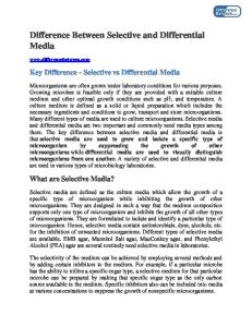
E-distance vs. ck-difference. The ck-difference is estimated by the size of the transformation program sTP. Figure 7 shows clearly that the e-distance and the ckdifference are not correlated when the transformation programs are simple (correlation coefficient 0.06 for sTP in [4,32]) and well correlated when the programs are complex (correlation coefficient 0.57 for sTP in [100,128]).

25

Figure 7. Size of the equivalent program p(S1, S2) versus e-distance e(S1, S2).

4.3

Discussion and interpretation

The previous results confirm that the e-distance e(S1, S2) is a good indicator of the number of changes really executed to transform S1 into S2. The relative difference is small, and is of the same order than the number of false positive in the case of random, independent sequences. On the other hand, the results show that the size of the transformation program can be used as a first approximation of the ck-difference. This was likely to occur in this particular case, because the repetitions of the loops are randomly chosen, and the spatial frequencies are random prime numbers (i.e. there is no clear pattern in the transformation program itself). Moreover, the difference between the number of changes and the number of operations executed by the transformation is small, in spite of the boundary effects (finite sequences cause several changes to occur at the same place). It is unlikely that this difference could be used to shorten the transformation program.

26

Finally, the foregoing conjecture is well illustrated by the experimental results. It can be seen that the e-distance bear no relationship with the estimate of the ck-difference when the transformation program has few loops, i.e. when it is simple to describe. On the contrary, when the transformation program has many loops, i.e. it is complex to describe, the e-distance is roughly proportional to the estimate of the ck-difference. This can be seen clearly on Figure 7, in spite of the noise introduced by the foregoing factors (false positive of the e-distance, and boundary effects).

27

5

CONCLUDING REMARKS

The edit distance is a useful tool, commonly used in important scientific fields, such as genomic computation. On the other hand, the Chaitin-Kolmogorov difference is an abstract concept, based on the theory of the informational complexity. By giving a common interpretation to these concepts, as an amount of work necessary to perform a transformation, a useful criterion is obtained, in order to choose the best way (manual or automatic) to perform a task. This could be applied to a broad range of tasks, any time that the input and the output of the task can be described by means of sequences (of symbols, characters, numbers, ...). However, much work remains to be done to determine the possible applications and the limitations of this approach, and to transform it into a set of practical decision tools.

28

REFERENCES Abrahamson, K. (1987). Generalized string matching. SIAM journal on computing, 16(6), 1039-1051. Bellman, R. (1957). Dynamic Programming. Princeton: Princeton University Press. Bellman, R. (1958). Dynamic programming and stochastic control processes. Information and Control, 1(3), 228-239. Brassard, G., Bratley, P. (1996). Fundamentals of Algorithms. New York: Prentice Hall. Chaitin, G. J. (1966). On the length of programs for computing binary sequences. Journal of the ACM, 13, 547-569. Chaitin, G. J. (1969). On the length of programs for computing binary sequences: statistical considerations. Journal of the ACM, 16, 145-159. Chaitin, G. J. (1974). Information theoretic limitations of formal systems. Journal of the ACM, 21, 403-424. Cormode, G., Muthukrishnan, S. (2001). The String Edit Distance Matching Problem with Moves. DIMACS Technical Report 2001-26. Cover, T.M., Thomas, J.A. (1999). Information Theory, in The MIT Encyclopedia of the cognitive sciences, Cambridge, MA.: Wilson & Keil editors, MIT press, 405-406. Crochemore M., Rytter, W. (1994). Text Algorithms. Oxford, UK.: Oxford University Press. Delahaye, J-P. (1994). Information, complexité et hasard. Paris: Hermès. Gusfield, D. (1997). Algorithms on Strings, Trees and Sequences: Computer Science and Computational Biology. New York: Cambridge University Press. Kolmogorov, A. N. (1965). Three approaches to the quantitative definition of information. Problems of Information Transmission, 1, 4-7. Levenshtein, V.I. (1966). Binary codes capable of correcting deletions, insertions and reversals. Soviet Physics Doklady, 10(8), 707-710. Masek, W.J., Paterson, M.S. (1980). A faster algorithm computing string edit distances. J. of Computer and System Sciences, 20, 18-31.

29

Smith, T.F. and Waterman, M.S. (1981). Identification of common molecular subsequences. Journal of Molecular Biology, 147, 195-197. Solomonoff, R.J. (1964). A formal theory of inductive inference. Information and Control, 7, 1-22, 224-254. Von Neuman, J. (1956). The General and Logical Theory of Automata. in James R. Newman editor, The World of Mathematics, Volume 4, New York: Simon and Schuster.

30