B.Sc. Engg. Thesis
Effect of Redundancy on Broadcasting in Untrusted Ad hoc Wireless Network by Syed Ashker Ibne Mujib Student No. 0305010
Arup Raton Roy Student No.: 0305059
Nashid Shahriar Student No.: 0305072
Submitted to Department of Computer Science and Engineering in partial fulfilment of the requirements for the degree of Bachelor of Science in Computer Science and Engineering
Department of Computer Science and Engineering Bangladesh University of Engineering and Technology Dhaka-1000
March 2009
Candidate’s Declaration This is to certify that the work presented in this thesis titled “Effect of Redundancy on Broadcasting in Untrusted Ad hoc Wireless Network” is the outcome of the investigation carried out by us under the supervision of Assistant Professor Dr. A.K.M. Ashikur Rahman in the Department of Computer Science and Engineering, Bangladesh University of Engineering and Technology (BUET), Dhaka. It is also declared that neither this thesis nor any part thereof has been submitted or is being currently submitted anywhere else for the award of any degree or diploma.
......................................... Syed Ashker Ibne Mujib Student No.: 0305010
......................................... Arup Raton Roy Student No.: 0305059
........................................ Nashid Shahriar Student No.: 0305072
Certificate The thesis titled “Effect of Redundancy on Broadcasting in Untrusted Ad hoc Wireless Network” submitted by Syed Ashker Ibne Mujib Student No.: 0305010, Arup Raton Roy Student No.: 0305059 and Nashid Shahriar Student No.: 0305072, has been accepted as satisfactory in partial fulfillment of the requirement for the degree of Bachelor of Science and Engineering in Computer Science and Engineering (B. Sc. Engg.) held on March, 2009.
Board of Examiner
................................................. Dr. A.K.M. Ashikur Rahman Assistant Professor Computer Science and Engineering Bangladesh University of Engineering and Technology (BUET) Dhaka-1000, Bangladesh
Contents Candidate’s Declaration
i
Certificate
ii
List of Figures
vi
List of Tables
vii
Acknowledgments
viii
Abstract
ix
1 Introduction 1.1
1
Mobile Ad hoc Network: MANET . . . . . . . . . . . . . . . . . . . . . . . . . .
2
1.1.1
Criteria . . . . . . . . . . . . . . . . . . . . . . . . . . . . . . . . . . . .
2
1.1.2
Usage . . . . . . . . . . . . . . . . . . . . . . . . . . . . . . . . . . . . .
4
1.2
Untrusted Environment . . . . . . . . . . . . . . . . . . . . . . . . . . . . . . . .
4
1.3
Motivation . . . . . . . . . . . . . . . . . . . . . . . . . . . . . . . . . . . . . . .
6
1.4
Our Contribution . . . . . . . . . . . . . . . . . . . . . . . . . . . . . . . . . . .
8
1.5
Document Structure . . . . . . . . . . . . . . . . . . . . . . . . . . . . . . . . .
9
2 Overview of Past Work 2.1
10
Classification of Broadcast Protocols . . . . . . . . . . . . . . . . . . . . . . . . 12 2.1.1
Unreliable Broadcast Protocol . . . . . . . . . . . . . . . . . . . . . . . . 13
iii
Contents
2.2
iv
2.1.2
Reliable Broadcasting Protocols . . . . . . . . . . . . . . . . . . . . . . . 14
2.1.3
Reactive and Proactive Protocols . . . . . . . . . . . . . . . . . . . . . . 18
Efficient Broadcasting Protocols in Untrusted Environment . . . . . . . . . . . . 19
3 Mitigating Misbehavior by Controlled Redundancy
21
3.1
Introduction . . . . . . . . . . . . . . . . . . . . . . . . . . . . . . . . . . . . . . 21
3.2
Preliminaries . . . . . . . . . . . . . . . . . . . . . . . . . . . . . . . . . . . . . 22 3.2.1
Notations . . . . . . . . . . . . . . . . . . . . . . . . . . . . . . . . . . . 22
3.2.2
Connected Dominating Set . . . . . . . . . . . . . . . . . . . . . . . . . . 22
3.2.3
The Dominant Pruning (DP) Algorithm . . . . . . . . . . . . . . . . . . 23
3.2.4
Forwardlist Creation Process . . . . . . . . . . . . . . . . . . . . . . . . . 23
3.2.5
The Partial Dominant Pruning (PDP) Algorithm . . . . . . . . . . . . . 24
3.3
Multiple Dominant Pruning (MDP) Algorithm . . . . . . . . . . . . . . . . . . 25
3.4
Redundancy versus Reachability: Untrusted Environment . . . . . . . . . . . . . 27
3.5
The Iterative Dominant Pruning (IDP) Algorithm . . . . . . . . . . . . . . . . . 29
3.6
3.5.1
Motivation . . . . . . . . . . . . . . . . . . . . . . . . . . . . . . . . . . . 29
3.5.2
Key Concept . . . . . . . . . . . . . . . . . . . . . . . . . . . . . . . . . 29
3.5.3
Iterative Dominant Pruning (IDP) Algorithm . . . . . . . . . . . . . . . 30
3.5.4
IDP and Misbehaving Node Detection Techniques . . . . . . . . . . . . . 31
3.5.5
IDP Applicability . . . . . . . . . . . . . . . . . . . . . . . . . . . . . . . 32
Demonstration with Example . . . . . . . . . . . . . . . . . . . . . . . . . . . . 32 3.6.1
Scenario . . . . . . . . . . . . . . . . . . . . . . . . . . . . . . . . . . . . 32
3.6.2
Simulation . . . . . . . . . . . . . . . . . . . . . . . . . . . . . . . . . . . 33
3.6.3
Outcome . . . . . . . . . . . . . . . . . . . . . . . . . . . . . . . . . . . . 39
Contents
v
4 Experimental Results
41
4.1
Performance Metrics . . . . . . . . . . . . . . . . . . . . . . . . . . . . . . . . . 41
4.2
Scenario Generation . . . . . . . . . . . . . . . . . . . . . . . . . . . . . . . . . 42
4.3
Traffic Generation . . . . . . . . . . . . . . . . . . . . . . . . . . . . . . . . . . . 43
4.4
Novelty of IDP . . . . . . . . . . . . . . . . . . . . . . . . . . . . . . . . . . . . 43
4.5
Graphical Comparison . . . . . . . . . . . . . . . . . . . . . . . . . . . . . . . . 43 4.5.1
Constant Pause Time . . . . . . . . . . . . . . . . . . . . . . . . . . . . . 43
4.5.2
Constant Percentage of Malicious Nodes . . . . . . . . . . . . . . . . . . 45
5 Conclusion and Future Work
57
5.1
Summary . . . . . . . . . . . . . . . . . . . . . . . . . . . . . . . . . . . . . . . 57
5.2
Future Work . . . . . . . . . . . . . . . . . . . . . . . . . . . . . . . . . . . . . . 58
Appendix
59
Bibliography
68
List of Figures 1.1
Conceptual Model of MANET . . . . . . . . . . . . . . . . . . . . . . . . . . . .
2
1.2
Trade-off between redundancy and reachability in untrusted environment . . . .
9
3.1
Connected Dominating Set . . . . . . . . . . . . . . . . . . . . . . . . . . . . . . 23
3.2
Scenario differentiating the approaches of PDP, DP, MDP-2, MDP-3 . . . . . . . 28
3.3
No Misbehaving Node . . . . . . . . . . . . . . . . . . . . . . . . . . . . . . . . 33
3.4
Single Misbehaving Node . . . . . . . . . . . . . . . . . . . . . . . . . . . . . . . 33
3.5
Two Misbehaving Nodes . . . . . . . . . . . . . . . . . . . . . . . . . . . . . . . 34
3.6
Four Misbehaving Nodes . . . . . . . . . . . . . . . . . . . . . . . . . . . . . . . 34
4.1
Packet Delivery Fraction with Varying Percentage of Misbehaving Node . . . . . 47
4.2
Normalized Efficiency with Varying Percentage of Misbehaving Node . . . . . . 48
4.3
Normalized Routing Load with Varying Percentage of Misbehaving Node . . . . 49
4.4
Average End to End Delay with Varying Percentage of Misbehaving Node . . . 50
4.5
Average Route Discovery Latency with Varying Percentage of Misbehaving Node 51
4.6
Packet Delivery Fraction with Varying Pause Time . . . . . . . . . . . . . . . . 52
4.7
Normalized Efficiency with Varying Pause Time . . . . . . . . . . . . . . . . . . 53
4.8
Normalized Routing Load with Varying Pause Time . . . . . . . . . . . . . . . . 54
4.9
Average End to End Delay with Varying Pause Time . . . . . . . . . . . . . . . 55
4.10 Average Route Discovery Latency with Varying Pause Time . . . . . . . . . . . 56 vi
List of Tables 3.1
Neighbors Within Two Hops . . . . . . . . . . . . . . . . . . . . . . . . . . . . . 35
3.2
Simulation of Non-adaptive Broadcasting Protocols : Single Cover . . . . . . . . 37
3.3
Simulation of Non-adaptive Broadcasting Protocols : Multiple Cover
3.4
Robustness of Non-adaptive Protocols in Presence of Misbehaving Nodes . . . . 40
3.5
Nodes Involved in Broadcasting . . . . . . . . . . . . . . . . . . . . . . . . . . . 40
3.6
Number of Attempts of IDP . . . . . . . . . . . . . . . . . . . . . . . . . . . . . 40
4.1
Distribution of Successful route-setup in iterations of IDP . . . . . . . . . . . . . 44
vii
. . . . . . 38
Acknowledgments
We would like to thank our supervisor Dr. A.K.M. Ashikur Rahman for introducing us in the arena of ad hoc networking and giving clear concept of this field. We express our heartiest gratitude to him for teaching us the procedure of carrying out research and suggesting the pathway of exploration addressing the untrusted ad hoc network. We are grateful to him for providing the valuable contents and giving lectures on NS-2 and gnuplot. We are also thankful to him for reviewing our drafts, correcting the proofs and giving his precious time and advice whenever needed. His continual encouragement acted as the source of inspiration and strength to perform this long time thesis; without which it would not be possible for us to complete this successfully. But his endless cooperation and support have made it an unyielding reality. Lastly, we are thankful to the NS-2 related tutorials, websites and mailing lists found on the internet and to the NS manual provided by the official team. These documentations have helped us to become familiar with NS-2 and thus to simulate the ideas of our research.
viii
Abstract Several protocols for broadcasting try to reduce redundancy as an effective measure against collision problems. Though these protocols guarantee good performance in a friendly environment, they fail to perform well when node cooperation cannot be enforced due to intentional misbehavior or environmental hostility. As a result, the expected behavior of nodes to forward packets, which is the basic assumption of all broadcast approaches, cannot be achieved always. In this research, we analyze the performance deterioration of these algorithms in hostile situation. As a remedy, we focus our intention in the reverse direction and interestingly find that adding redundancy in a controlled manner can greatly compensate the performance degradation due to node misbehavior. Here, we propose a new approach called Iterative Dominant Pruning (IDP) that tune the amount of redundancy so that reachability and routing load both remain at a satisfactory level. Simulation results of applying different broadcast algorithms show significant performance improvement in the case of Iterative Dominant Pruning. Based on the observations, we discuss applicability of Iterative Dominant Pruning and scope of its further improvement. Comparing their relative performance, we end up with the conclusion that though redundancy is undesired, controlled redundancy is effective in special situations like unfavorable environments.
ix
Chapter 1 Introduction The necessity of information is obligatory and means of communication is vital from the dawn of the civilization. In communication, like all other fields, the requirement of society continuously increases with time. Scientists invented newer techniques to keep pace with the changed need. Wired network was the first approach. Now-a-days, the mainly three basic systems people use to set up wired networks: Ethernet, phone line and broadband. Due to the low cost, high security and already created infrastructure (especially for phone line) wired network is still popular. Communication technology evolved from wired to wireless. The rapid advances of radio technology in the 1970’s stimulated the development of mobile communications. The flexibility to adapt to mobile environments results in the widespread acceptance and popularity of wireless networks. On the heel of the success of cellular telephony came the interest to connect to the Internet from mobile terminals. Due to the differences found in the physical layer of these systems, wireless devices and networks show distinct characteristics from their wireline counterparts, specially, higher interference, lower reliability, lower speed, highly variable network conditions, higher jitter, higher data loss, frequent disconnection etc. Conventional wireless networks require as prerequisites a fixed network infrastructure with centralized administration for their operation. Recent developments in ad hoc wireless networking have eliminated the requirement of fixed infrastructure for communication between users in a network. This expanded the horizon of wireless networking.
1
Introduction
2
Figure 1.1: Conceptual Model of MANET
1.1
Mobile Ad hoc Network: MANET
MANETs are a collection of autonomous terminals that communicate with each other by forming a multihop radio network and maintaining connectivity in a decentralized manner. In such a network, each mobile node operates not only as a host but also as a router by finding routes and forwarding data packets for other nodes while remaining mobile. A conceptual model of MANET can be illustrated in Figure: 1.1 [19].
1.1.1
Criteria
MANETs inherit common characteristics found in wireless networks in general. But MANET has distinguished features other than those. These salient features can be stated as follows: • Mobility : Infrastructure-less network provides facility of mobility to the host. Mobility can be of various forms like random mobility, group mobility, motion along preplanned
Introduction
3
route etc. The mobility model has major impact on the selection on routing scheme and thus influences performance. • Multi-hopping : Multi-hop networks use two or more nodes to convey information from a source to a destination. Ad hoc networks often exhibit multiple hops for obstacle negotiation, spectrum reuse and energy conservation. • Self-organization: The ad hoc network must autonomously determine its own configuration parameters such as addressing, routing, clustering, position identification, power control, etc. Special nodes (e.g., mobile backbone nodes) can coordinate their motion and dynamically distribute in the geographic area to provide coverage of disconnected islands in some cases. • Energy Conservation: Most nodes in ad hoc network have limitation in power supply. Energy efficient protocol design (e.g., MAC, routing, resource discovery etc) is critical for prolonged existence. • Scalability : The ad hoc network can grow to several thousand nodes in some applications like large environmental sensor fabrics, battlefield deployments, urban vehicle grids, etc. For wireless “infrastructure” networks, scalability is simply handled by a hierarchical construction. The limited mobility of infrastructure networks can also be easily handled using Mobile IP or local handoff techniques. In contrast, because of the more extensive mobility and the lack of fixed references, pure ad hoc networks do not tolerate mobile IP or a fixed hierarchy structure. Thus, mobility, jointly with large scale is one of the most critical challenges in ad hoc design. • Security : The challenges of wireless security are well known - ability of the intruders to snoop around and jam the channel. The ad hoc networks are more vulnerable to attacks than the infrastructure counterparts. Both active and passive attacks are possible. An active attacker tends to disrupt operations. Due to the complexity of the ad hoc network protocols, these active attacks are by far more difficult to detect in ad hoc than infrastructure nets. Passive attacks are unique of ad hoc nets, and can be even more dangerous than the active ones. Eventually, the active attacker is discovered and
Introduction
4
physically eliminated. The passive attacker is never discovered by the network. It is placed in a sensor field or at a street corner like a bug, monitoring data and control traffic patterns. The information is relayed back to the enemy headquarters via special communications channels with low energy and low probability of detection. Defense from passive attacks require powerful novel encryption techniques coupled with careful network protocol designs.
1.1.2
Usage
In situations, where there is little or no communication infrastructure or the existing infrastructure is destroyed or inconvenient to use, or setting up a new fixed network for a transient period is too expensive an ad hoc wireless network can be a solution. The ad hoc wireless network have a wide variety of applications ranging from military in battlefields, commercial applications, emergency disaster and rescue areas, to networks for interactive conferences and wilderness expeditions. Applications of ad hoc wireless networks can be summarized as below: • Community Network • Enterprise Network • Home Network • Emergency Response Network • Vehicle Network • Sensor Network
1.2
Untrusted Environment
The implementations of all the established broadcasting approaches designed for MANET implicitly assumes that all nodes in the network cooperate in the communal task of maintaining connectivity. This assumptions need not be always valid; the properties of the ad hoc networks gives rise to several problems for a node to act as expected. The ad hoc networks established
Introduction
5
to serve special situations, intensify the problem to a much higher degree. So, there are such situations where a node may misbehave by agreeing to forward packets and then failing to do so, because it is overloaded, selfish, malicious, or broken. These unexpected behavior of nodes can be classified as follows: • Overloaded Node: An overloaded node lacks the CPU cycles, buffer space, or available network bandwidth to forward packets. This overloading may happen in the dense part of the network, where a node is involved in handling too much data and network packets beyond its capacity. • Selfish Node: A selfish node is one that wants to get a free ride without contributing to the neighboring community. Such a node is unwilling to spend battery life, CPU cycles, or available network bandwidth to forward packets not of direct interest to it, even though it expects others to forward packets on behalf of it. • Malicious Node: A malicious node launches a denial of service attack by dropping packets. Such a harmful node might want to draw attention to itself by advertising many bogus neighbors, thus posing for a highly relevant node. These type of nodes might be present on the network having the clear intention of conveying wrong messages or damaging the reliability of the network channel. • Broken Node: A broken node might have a software fault, hardware damage, or suffering from blackout that prevents it from forwarding packets. Again, some nodes may be actually misbehaving or they may bona-fide fail to carry out their tasks due to some error or hostile situation. Arguably, the two cases are different and thus seek for different type of treatment to handle their failure. An intentionally misbehaving node may try to mislead its neighbors, e.g., by acknowledging packet and then dropping it at certain times, or by deceiving its neighbor by agreeing to forward packets and then failing to do so. On the other hand, honest and continuous unintentional failure may be easier to diagnose by the network and thus easier to recover from. Our concern is the intentional misbehavior which can also happen for some other reasons except harmful attitude. Such case might be- a
Introduction
6
node may agree to forward a packet and then fail to forward it for objective reasons, e.g., the target neighbor has already become temporarily unreachable because of interference or other environmental factors. So, throughout this dissertation we assume by untrusted environment, an ad hoc network having misbehaving nodes which remain in the neighbor list thus agreeing to forward packets then intentionally dropping the packet when required. Misbehaving nodes in untrusted environments can be a significant problem. The simulation results in [18] show that if 10% − 40% of the nodes in the network misbehaves, then the average throughput degrades by 16% − 32%. However, the worst case throughput experienced by any one node may be worse than the average, because nodes that try to route through the misbehaving node experience high loss while other nodes experience no loss. Thus even a few misbehaving nodes can have a severe impact on the network performance.
1.3
Motivation
A major challenge in the design of ad hoc network is the development of dynamic routing protocols that can efficiently find routes between two communicating hosts. There are two basic data exchange modes-unicasting and broadcasting. Issues related to routing are reduction of routing load, radio power limitation, proper channel utilization, performance deterioration due to low bandwidth of wireless links, security concerns etc. Optimum solutions for these problems exist in a variety of approaches. But majority of these approaches rely on the assumption that they are operating on cooperative environment. That is, they trust each node by assuming that a node will obviously forward a packet when requested to do so. In reality, it is difficult to expect and maintain a favorable environment for an ad hoc network, as such networks are created on the fly to circumstance some sort of unexpected situation. None of the protocols considers the problems associated with an untrusted and hostile environment where a node might misbehave, thereby violating the assumption of mutual cooperation. As discussed in 1.2, such environments may be consisted of nodes which are malicious, selfish [18] or even intentionally uncooperative and harmful [24] or unreachable due to mobility. Due to the host mobility and dynamic change of network topology in ad hoc wireless networks, broadcast routing are performed more frequently and expected to be more efficient.
Introduction
7
Several routing protocols such as Ad Hoc On-Demand Distance Vector routing (AODV) [22], Dynamic Source Routing (DSR) [13] rely on broadcast to obtain routing information. Moreover, broadcasting is a common and fundamental operation in many applications e.g. graph related problem, distributed computing, multicast service in wired networks. One straightforward and obvious approach for broadcasting is blind flooding, in which each node will rebroadcast the packet whenever it receives it for the first time. Blind flooding generates many redundant transmissions and thus increases the routing load on the network. Uncontrolled flooding leads to a more serious broadcast storm [20] problem which is caused by serious redundancy, contention and collision in the network. Therefore, it is always the rational tendency of broadcast algorithm designers to cut down the redundancy by proposing efficient flooding algorithms [2], [4], [16], [20], [21], [23], [26]. The Dominant Pruning (DP) [16] is one of the promising approaches that utilizes neighborhood information to reduce redundant transmission. Though, DP is considered as the extreme counterpart of blind flooding, further improvement is possible which utilizes neighbor information more effectively. The Total Dominant Pruning (TDP) [17] and Partial Dominant Pruning (PDP) [17] are two such approaches that deal with the deficiency of DP and result to even more controlled broadcast. While designing a broadcast protocol for ad-hoc networks, one of the primary goal is to reduce the number of retransmission, specially redundant retransmission while reaching all the nodes in the network. Another important goal is to ensure that all the desired nodes within the network receives the message in spite of reducing number of retransmission. This significant goal is not achieved by the above broadcast approaches in the untrusted environments due to lacking of effort and concentration imposed on this type of behavior. But such unwanted situations come into existence in most of the ad hoc networks. With the rapid advancement of ad hoc networks and wide variety of its usage, it is the high time to give more emphasis on the analysis of broadcast algorithms from untrusted perspective.
Introduction
1.4
8
Our Contribution
Although eliminating redundant transmission is obvious in friendly, cooperative environment but may not be effective in untrusted, hostile environment. The reason is, controlled broadcasts rely heavily on some nodes of the connected dominating set [15] by trusting each node equally. If one such node somehow misbehaves, that may create a partition in the network and thus may deny to achieve the goal of the operation. As a remedy, another variant- Multicover Dominant Pruning (MDP), that relaxes the redundancy control of DP to compensate the performance loss caused by misbehaving nodes is proposed in [24]. One of the contributions of our research is to analyze the performance of DP and its variants (i.e. PDP, TDP and MDP) in untrusted scenarios. For illustration, the broadcast component of a popular routing protocol AODV is modified to incorporate these broadcasting techniques. In this research, we also investigate a basic but important issue of broadcasting–the trade-off between redundancy and reachability aspects as illustrated in Figure 1.2. Through simulation we show that under the assumption of cooperative environment, redundancy degrades network performance. However, in a hostile environment where vicious nodes exists, redundancy cutdown causes a significant loss in the global reachability. Our analysis shows, adding redundancy in a controlled way in such situations upgrades the performance (i.e. increases reachability). These behavior urges us either to compromise between these two aspects or to go for a novel technique that integrates the advantage of both. Considering this trade-off, we propose an adaptive approach Iterative Dominant Pruning (IDP) that optimizes the above aspects irrespective of the environment. This scheme adapts with the situation by increasing the number of broadcasts only when needed, keeping it to a minimum value in friendly situations. IDP differs from the already established approaches applicable to MANET in the respect that the previous versions focus mainly on one direction of the broadcast problems that is either to attain high rechability or to cutdown redundancy, whereas IDP targets to achieve both goal optimally. We do not however analyze any killer application of IDP in this research. Rather our vision is merely to illustrate a light-weight simplistic technique in hostile environment. As part of our thesis work, we also developed a tutorial website on the wireless portion of Network Simulator-2 (NS-2), a widely used simulator for network related researches. The goal
Introduction
9
Redundancy Cutdown
Environment Reachability Hostility
Figure 1.2: Trade-off between redundancy and reachability in untrusted environment of the website is to help the beginners who want to use NS-2 as part of their work but facing problems initially. The adress of the site is: http://teacher.buet.ac.bd/ashikur/ns2/
1.5
Document Structure
This chapter provides a brief introduction to ad-hoc wireless networks, the motivation behind our research and the ultimate goals and contribution of this research. Chapter 2 provides a summary of relevant related works to the problems in which we are interested. Chapter 3 briefly summarizes DP, PDP, MDP and IDP algorithms. This chapter mainly focuses on the details of our proposed findings and IDP algorithm. Next, chapter 4 includes examples demonstrating the major differences and working principle of variants dominant pruning algorithm. These examples exhibits the behavior of these algorithms in the untrusted environment from the perspective of reachability and redundancy. A detailed experimental result showing the effectiveness of our proposed scheme is also presented in chapter 5. Finally, chapter 6 concludes and points out some future work based on this research.
Chapter 2 Overview of Past Work In an ad-hoc network, several types of transmitting operations might be needed. Some of those can be: Unicasting, Multicasting, Broadcasting. Among these, Broadcasting plays the most fundamental role. Whenever a sender broadcasts a packet, all nodes within its transmission range is effected by this transmission. In a nutshell, broadcasting means, a source node transmits the same message to all the nodes within the network. In one-to-all model, message transmitted by one node will reach all nodes that are within the transmission radius of that node. On the other hand, in one-to-one model, each transmission is directed towards only one neighbor node. In literature, broadcasting has been studied for mainly one-to-all model and throughout this dissertation we will also devote to that model. Despite its many usefulness, the biggest disadvantage of Broadcasting is that it interferes with the sending and receiving of other transmissions. This problem is referred to as exposed node problem, that is an outgoing transmission collides with incoming transmission and hidden node problem, that is two incoming transmissions collide with each other. Broadcasting is often necessary in route discovery or service discovery in many on demand routing protocols. Routing protocols for MANET can be classified as proactive and reactive, depending on how they react to topology. In case of proactive routing protocols, nodes interchange routing information periodically in order to maintain consistent and accurate routing information. When a node needs to transmit data to a destination, it can rapidly compute the path based on the available updated information of the routing table. Thus proactive routing protocols use broadcasting for exchanging routing information with other nodes. But the 10
Overview of Past Work
11
negative side of proactive routing protocol is that it requires high overhead to exchange and maintain an up to date routing table. In ad hoc wireless networks, node mobility triggers a dynamic topology that might require a large number of routing updates. This has a negative impact on resource constrained wireless devices, bandwidth utilization and throughput. Observing that the proactive protocols wastes limited wireless bandwidth, many researchers have proposed reactive protocols, in which only on-demand routes are created. Reactive routing protocols uses broadcasting to discover a route from the source node to the destination node. Another application of broadcasting can be in detection of location, where location-aware routing can be used. Also, recent advances in technology have made it possible to integrate micro-sensor, low power signal processing, computation and low cost wireless communication in a sensing device. Furthermore, there exists other application of MANET in which broadcasting plays a fundamental and significant role. Therefore, optimal broadcasting in mobile ad hoc networks is crucial for providing services in different application. In general, broadcasting refers to a process of transmitting a packet so that all nodes within the network receives a copy of this packet. Flooding is the most common and simple approach for broadcasting where every node in the network forwards the packet exactly once. In flooding, it is guaranteed that all nodes within the network will receive a broadcasted packet, provided that the network is connected, static and the underlying MAC layer is ideal. But such a straightforward implementation of broadcasting is usually very costly, and results in serious redundancy, contention, and collision, which is referred to as broadcast storm problem [20]. When the size of the network increases and the network becomes dense, more transmission redundancy will be introduced and ultimately it will result in broadcast storm problem. To implement our proposed approach we choose one of the mature algorithms for ad hoc network routing, AODV which exploits broadcasting. In AODV, when a node attempts to send a data packet to a destination, it uses route discovery process to find such a route. The discovery process starts by initiating a route request (RREQ) which is flooded blindly over the network. Each node upon receiving RREQ, rebroadcasts it, unless it is the destination or it has a route to the destination in its cache. The destination itself or any node in the path that
Overview of Past Work
12
contains the route then sends a route reply (RREP) to establish the route. The blind flooding used in AODV gives rise to several problems as mentioned earlier in this chapter. Some of the approaches against blind broadcasting are probabilistic [20] in nature, so they cannot guarantee all the nodes in the network receiving the broadcast packet. Another approach DP, gives this guarantee of reaching all the nodes while cutting down the number of broadcast transmission to a great extent. To achieve this, each node finds a subset of its one-hop neighbors which is called forward list. In the next hop, only the nodes in the forward list rebroadcast the packet to the two-hop nodes. Even more reduced broadcast techniques are PDP and TDP which utilize neighborhood information more effectively. PDP drops out the one-hop neighbors of common neighbors of both sender and receiver of a broadcast packet from the list of nodes to be covered. Similarly TDP drops the two-hop neighbors of the sender from that list. This requires extra three-hop neighbor information piggybacked in broadcast packet of TDP, which increases overhead. DP, PDP, TDP compute the forward node list in such a way that all two-hop neighbors are covered by the rebroadcast of at least one direct neighbor node. Though DP and its variants perform well in normal case, they suffer in the untrusted situations. In these environments, redundant broadcasts like MDP can be an effective solution. The idea behind MDP is to introduce redundancy in broadcasting to increase reachability without detecting or specifically identifying which nodes are misbehaving.
2.1
Classification of Broadcast Protocols
More than a decade have passed on broadcast optimization research and several techniques have been proposed [14, 16, 17, 20, 21]. Broadcast algorithm can be broadly classified as reliable and unreliable algorithms, which are also referred to as probabilistic and deterministic algorithms respectively. A reliable broadcast algorithm may work as unreliable algorithm if the underlying MAC layer does not work perfectly or other types of imperfection occurs. But considering an ideal MAC layer, we can call a broadcast algorithm reliable if it guarantees that a broadcast message reaches all nodes in the network. On the other hand, if a broadcast protocol cannot guarantee that a message reaches all nodes within the network or depend on a probability, it
Overview of Past Work
13
is called unreliable broadcast protocol.
2.1.1
Unreliable Broadcast Protocol
In this type of broadcast protocol, whenever a node receives a broadcast packet, it forwards the packet with probability P . The value of P is determined depending on the available relevant information at that node. Though this approach provides good stochastic result, it cannot guarantee full coverage of nodes. Different types of probabilistic broadcasting approaches are described in [20]. Enhancement of this techniques were also addressed in [5, 9]. Some unreliable broadcasting approaches are: • Probabilistic Scheme • Counter Based Scheme • Distance Based Scheme • Location Based Scheme The broadcast storm problem generated by simple flooding can be avoided by reducing the number of nodes that retransmit the broadcast packet. The unreliable approach tries to solve this problems of simple flooding method. Next we present a brief description of different unreliable broadcasting approaches. • Probabilistic Scheme: An intuitive way to reduce rebroadcast is to use probabilistic rebroadcasting where on receiving a broadcast message for the first time, a host will rebroadcast it with probability P . When P = 1, this scheme is equivalent to flooding. To take measure against contention and collision problems, we should introduce a small random delay before rebroadcasting the message so that the timing of rebroadcasting can be differentiated. • Counter Based Scheme: Upon the reception of a previously unknown packet, the node initiates a waiting timer and a counter. The counter increases one for each received redundant packet. When the waiting timer expires, if the counter is larger than a threshold value, the node will not rebroadcast the packet; otherwise, the node will broadcast it.
Overview of Past Work
14
• Distance Based Scheme: Upon receiving a previously unknown packet, the node initiates a waiting timer. Before the waiting timer expires, the node checks the location of the senders of each received redundant packet. If any sender is closer than a threshold distance value, the node will not rebroadcast the packet. Otherwise, the node rebroadcasts it when the waiting timer expires. • Location Based Scheme: When a previously unknown packet is received, the node initiates a waiting timer and accumulates the coverage area that has been covered by the arrived packets. When the waiting timer expires, if the accumulated coverage area is larger than a threshold value, the node will not rebroadcast the packet. Otherwise, the node will broadcast it.
2.1.2
Reliable Broadcasting Protocols
The reliable approach provides full coverage of the network for a broadcast operation. Here, only a subset of nodes forward the broadcast packet and the remaining nodes are adjacent to the nodes that forward the packet. The nodes that forward the broadcast packet form a forward node set for a particular broadcast operation. Basically, a forward node set is a connected dominating set (CDS). A dominating set (DS) is a subset of nodes such that every node in the graph is either in the set or is adjacent to a node in the set. If the subgraph induced from a DS of the network is connected, the DS is a CDS. To achieve hundred percent reachability, only the nodes in a connected dominating set (CDS) are required to retransmit. Therefore, the optimal broadcast problem can be solved by finding a connected dominating set of minimum size i.e MCDS. But finding a minimum connected dominating set (MCDS) in a given graph is NP-complete [16]. So finding approximation algorithm is an alternate solution to this problem. Approximation algorithms with a constant approximation ratio can easily be derived. On the other hand, finding an approximation algorithm with a small constant approximation ratio is still a challenging issue in the absence of global network information [4]. If global network topology information is available, then approximation algorithms proposed in [7] can be used to solve the problem of MCDS. But the main flaw of this algorithm is, it requires global network information. In wireless ad hoc network, topology may change
Overview of Past Work
15
drastically due to the dynamic nature of nodes. Therefore, many heuristic algorithms were proposed that can compute connected dominating sets in distributed fashion based on local information only. All distributed heuristics seek a small forwarding set with the least possible overhead. Different types of deterministic broadcasting heuristics are: • Simple Flooding • Self Pruning (SP) • Dominant Pruning (DP) • Multi Point Relaying • Total Dominant Pruning (TDP) • Partial Dominant Pruning (PDP) • Enhanced Partial Dominant Pruning (EPDP) • Cluster Based Algorithm • Scalable Broadcasting Algorithm (SBA) There are numbers of research literature that propose countless efficient deterministic broadcasting techniques whose ultimate aim is to minimize number of retransmissions. In this section we analyze different heuristic algorithms which directly or indirectly aims at reducing the number of broadcasting. • Simple Flooding : Simple flooding is the common method for broadcasting in which each node rebroadcasts to its neighbors whenever it receives a message. The enormous number of redundant broadcast packets which occurs due to pure flooding is referred to Broadcast Storm Problem[20]. According to the authors one way to optimize flooding is to take an unreliable approach. Some of the unreliable approaches were discussed in section 2.1. These schemes mainly differ on two issues: One is how the mobile nodes calculate redundancy. And the other is: how this calculated expertise facilitates nodes to
Overview of Past Work
16
assist its decision. One of the main problem of these algorithms is they cannot guarantee enough reachability. Note also that a protocol that is reliable on the network layer may be very unreliable at the MAC layer, such as blind flooding. • Self Pruning (SP): The fundamental criteria of Self Pruning [16] requires that each node have knowledge of its 1-hop neighbors. Each node in this approach is required to have knowledge of its neighbors, this knowledge can be achieved by periodic Hello messages. The receiving node will first compare its neighbor lists to that of senders list, the receiving node will rebroadcast if the additional nodes could be reached, otherwise the receiving node will drop the message. This is the simplest approach in the neighbor knowledge method. • Dominant Pruning (DP): Dominant Pruning uses 2-hop neighborhood information. In Dominant Pruning, it is required to choose some or all the nodes within 1-hop as rebroadcast nodes [16]. Only these chosen nodes are allowed to rebroadcast. Nodes inform neighbors to rebroadcast by including their address as part of a list in each broadcast packet header. Whenever a node receives a broadcast packet, it checks whether its address is contained within the list. If it exists, this node uses a greedy set cover algorithm to determine which subset of nodes should rebroadcast, depending on the available information about which neighbors have already been covered by sender’s transmission. This process continues until all nodes in the network receive the message. • Multi Point Relaying : Multi Point relaying [23] is similar to Dominant Pruning in that rebroadcasting nodes are explicitly chosen by upstream nodes. The chosen nodes are called Multi Point Relays (MPRs) and they are the only nodes allowed to rebroadcast a packet received from an upstream node. Each MPR is required to choose a subset of its 1-hop neighbors to act as MPRs as well. A node includes a neighbor in its MPR set only if it is the only neighbor in route to a two hop neighbor. The node iteratively includes all such neighbors in the MPR set. Then it picks a neighbor which is not already included in the MPR set and which covers the most 2-hop nodes that are uncovered by any member of the current MPR set. The last step continues until all 2-hop neighbors are covered by some member of the MPR set.
Overview of Past Work
17
• Total Dominant Pruning (TDP): Total Dominant Pruning (TDP) [17] make efficient use of neighborhood information. In Total Dominant Pruning, two-hop neighborhood information of the source is piggybacked within the packet and broadcast. A node receiving this message selects forward nodes based on the piggyback information. The main drawback of TDP is it requires high bandwidth as with every packet neighborhood information of the source is piggybacked. • Partial Dominant Pruning (PDP): Partial Dominant Pruning (PDP), proposed in [17], also makes efficient use of neighborhood information. In Partial Dominant pruning, neighborhood information of the source is not piggybacked within the broadcast packet. And its key idea is to reduce the number of 2-hop neighbors to be covered, which eventually reduces number of forward nodes. This is done by excluding the neighbors of common neighbors of both receiver and sender from the 2-hop nodes to be covered. One big advantage of PDP over TDP is that it has a reduced packet size. • Enhanced Partial Dominant Pruning (EPDP): Enhanced Partial Dominant Pruning (EPDP), proposed in [11], defers the rebroadcast to gather more information about neighborhood. During this defer time, if receiver node receives the same broadcast from nodes other than the sender, then the latter nodes and the neighbors of common neighbors of both receiver and latter nodes may be excluded from the list computed in PDP. This heuristic is very effective in reducing number of rebroadcasts with a slight increase in broadcast latency. • Cluster Based Algorithm: Although cluster-based broadcast algorithms are not local algorithms, they usually work well with local state information and low time delay. Basically, the clustered network converts any dense network to a sparse one consisting of clusterheads only since clusterheads form a DS of the network. Moreover, clusterheads and gateways form a CDS of the network. Therefore, this is enough to fulfill a broadcast operation when all clusterheads and gateways forward a broadcast packet. clustering approach has been used to address traffic coordination schemes [8] and routing problems [8]. • Scalable Broadcast Algorithm (SBA): The Scalable Broadcast Algorithm (SBA)
Overview of Past Work
18
[21] requires that all nodes have knowledge of their neighbors within two hop radius. All nodes can accomplish 2-hop neighborhood information by periodically generating “Hello” messages. Node’s identity along with this two hop neighborhood information is used to determine whether rebroadcasting is necessary or not. The key idea of this algorithm is that, a node need not rebroadcast a message if all its neighbors have been covered by previous transmissions. Here, the authors proposed that redundant rebroadcast can be circumvented by local topology information and knowledge of duplicate rebroadcasts. Moreover, a random delay is linked with each node which helps to reduce redundant rebroadcast further.
2.1.3
Reactive and Proactive Protocols
Depending upon the way of utilizing the neighborhood information to reduce the redundant rebroadcasts, we broadly classify the assortment of broadcast algorithms into two categories in this dissertation: • Reactive Protocols • Proactive Protocols • Reactive Protocols: In this protocol, each node makes its own forwarding decision after receiving a broadcast from a upstream node. To make such a decision, a node at first determines whether further forwarding is going to cover any more new nodes or not. If it seems to cover no more new nodes then it avoids forwarding. One of the most promising reactive broadcasting technique called Self Pruning (SP) was proposed in [16]. • Proactive Protocols: In proactive broadcasting, a node selects a subset of downstream nodes among its neighbors as forwarding nodes. A node tries to select most promising neighbors based on some criterion such as high node degree, power level, coverage area etc. Some promising examples of proactive approaches include Dominant Pruning (DP) [16], Partial Dominant Pruning (PDP) [17], Total Dominant Pruning (TDP) [17] etc. DP, TDP and PDP reduce redundant transmission by reducing the number of forward nodes.
Overview of Past Work
19
However, the impact of broadcast latency requires a thoughtful consideration for effective proactive broadcasting.
2.2
Efficient Broadcasting Protocols in Untrusted Environment
Most of the previous works addressing node misbehavior has been focused on unicast routing protocols [3], [10], [12], [13], [22]. Very few research aimed at broadcasting. All the aforementioned protocols are designed for trusted environment and they perform fairly well in those cases. But node cooperation cannot always be guaranteed which results in uncooperative or untrusted environment. Nodes may not show intended behavior because it may be temporarily down, it may want to save its battery power, it may show false neighbors or it may be malicious at the worst case. In all these cases, even the reliable protocols cannot yield sufficient coverage. This is due to the fact that controlled broadcasts, which cuts down redundancy to a great extent, rely heavily on some nodes of the Connected Dominating Set by trusting each node equally. If one such node somehow misbehaves, a disconnected partition in the network graph may be created and thus the goal of the operation may not be acheived. To give some resistance against malicious attacks, three types of protective schemes worth mentioning: cryptographic, incentive based and punishment based. Punishment based scheme is the most effective one among these and a special implementation of this scheme is proposed in [18]. Here, in each node, two specials tools, watchdog and rater is used. The watchdog monitors the behavior of all nodes on the active paths, and the rater allows the nodes to avoid paths leading through misbehaving nodes. Another effective approach called MDP is proposed in [24]. The idea behind MDP is to introduce redundancy in broadcasting to increase reachability without detecting or specifically identifying which nodes are misbehaving. By adding redundancy, multiple path is created between source and destination pairs. So even if one path contains untrusted intermediate nodes, the other paths ensures safe delivery. It is quite clear that in an uncooperative environment, reachability will increase with increasing redundancy. But it should be limited to a certain amount so that broadcast storm problems might not occur. The idea behind MDP is further
Overview of Past Work illustrated in Chapter 3.
20
Chapter 3 Mitigating Misbehavior by Controlled Redundancy 3.1
Introduction
The main outcome of our research is the establishment of the idea of controlled redundancy, which is effective for broadcasts in any environment including noncooperative environment. Our analysis provides a valid ground on which the technique of adding redundancy becomes obvios in untrusted situation. Working on this motivation, our main contribution is to find a way to incorporate right amount of redundancy at the right time. This finding leads us to propose a different scheme, Iterative Dominant Pruning (IDP) which adaptively employs appropriate amount redundancy based on the necessity. As this scheme makes use some of the already established variants of Dominant pruning, we first explain the working principle of dominant pruning. Before moving into IDP, we focus on the relevant broadcasting scheme on which our algorithm hinges. Then, we present modified version of Multiple Dominant Pruning (MDP) in a way that incorporates variants of DP in a single routine and is suitable to be used in our proposed IDP. We also analyze the different techniques of broadcasting on redundancy and rechability aspects. Arguments presented here are supported by the simulation results in the later chapter. Based on all these explanations, the concept of IDP, its applicability, advantages over the node detection methods, and elaborative examples are presented finally.
21
Mitigating Misbehavior by Controlled Redundancy
3.2 3.2.1
22
Preliminaries Notations
To illustrate our idea, let us assume that node v has just received a broadcast packet from node u and v is on u’s forward list Fu . Each node u determines the so called forward list as a subset of its one-hop neighbors whose transmissions will cover all two-hop neighbors. Thus when transmitting a broadcast packet, u explicitly indicates that it should be rebroadcast only by the nodes on the forward list. Now node v has to compute its own forward list Fv to be inserted into the header of the rebroadcast copy. Let N (u) be the set of all one-hop neighbors of node u. By N (N (u)) we shall denote the set of all one-hop and two-hop neighbors of u, i.e., N (N (u)) = {v|v ∈ N (u) ∨ ∃z[v ∈ N (z) ∧ z ∈ N (u)]} Throughout the chapter we assume that u (sender) and v (receiver) are neighbors. The way we used to collect two-hop neighbor information is to send simple hello messages with the time to live(TTL) of 2 periodically. Such a message will be rebroadcast exactly once and thus propagated to al two-hop neighbors of the sender.
3.2.2
Connected Dominating Set
Connected Dominating Set (CDS) S can be defined as ∀u [u ∈ S ∨ ∃v [v ∈ S ∧ u ∈ N (v)]] The Minimum Connected Dominating Set (MCDS) is the CDS with minimum cardinality. Any reliable broadcast guarantees a broadcast packet to reach every node in the network. Thus, every node in a particular CDS, S of the network must rebroadcast to obtain 100% reachability. To incorporate minimum number of rebroadcast, we should emphasis on finding the MCDS of the nodes of network. In Figure 3.1, some possible connected dominating sets are {A, C, E}, {A, E, G, H}, {B, D, F, I} etc. We cannot find any connected dominating set of size less than 3. Therefore, the (MCDS) of Figure 3.1 is {A, C, E}.
Mitigating Misbehavior by Controlled Redundancy
A
B
23
D
E
G
F
C
I
H
Figure 3.1: Connected Dominating Set
3.2.3
The Dominant Pruning (DP) Algorithm
Unfortunately, finding a minimum connected dominating set (MCDS) is NP-hard[6]. But there are some greedy approaches which can be considered as the approximation to the MCDS problem. Dominant Pruning is one of the heuristic algorithms which is a reliable broadcast protocol ensuring that a broadcast packet is guaranteed to reach every node in the network along with reducing redundant transmissions. Viewed as flooding containment scheme, dominant pruning limits its population of forward nodes to the connected dominating set with the aid of the two-hop neighbor information. The Dominant Pruning works on finding the minimum sized forward list to ensure reliable transmission. In this greedy approach, each node v determines the so-called forward list as a subset of its one-hop neighbors whose transmissions will cover all two-hop neighbors of v. Then, when transmitting a broadcast packet, v explicitly indicates that it should be rebroadcast only by the nodes on the forward list. Suppose that v has just received a packet from node u. The packet’s header includes the forward list Fu inserted there by u. The case v 6∈ Fu is simple: the node will not rebroadcast the packet; otherwise, v has to create its own forward list Fv to be inserted into the header of the rebroadcast copy. The following subsection describes how node v creates the forward list Fv .
3.2.4
Forwardlist Creation Process
To compute forward list, each node starts by constructing Uv , which is the set of uncovered two-hop neighbors of v. This set includes all two-hop neighbors of v that have not been covered
Mitigating Misbehavior by Controlled Redundancy
24
by the received packet, i.e., Uv = N (N (v)) − N (v) − N (u). Note that every node knows the population of its two-hop neighbors; thus, N (u) is known to v. Then, v sets Fv = φ and B(u, v) = N (v) − N (u). The set B(u, v) represents those neighbors of v which are possible candidates for inclusion in Fv . Then, in each iteration, v selects a neighbor w ∈ B(u, v), such that w is not in Fv and the neighbors of w covers the maximum number of nodes in Uv , i.e., |N (w) ∩ Uv | is maximized. Next Fv and Uv are updated. Fv = Fv ∪ {w} and Uv = Uv − N (w). The iterations continue for as long as Uv becomes nonempty or no more progress can be accomplished (i.e., there is no way to further improve the coverage).
3.2.5
The Partial Dominant Pruning (PDP) Algorithm
The most effective way to improve DP algorithm is to reduce the size of the forward list created by each node as the broadcast progresses. One such technique called PDP algorithm is mentioned in Chapter 2. The basic idea is to reduce the size of Uv set (i.e., reduce the number of two-hop neighbors to be covered). To achieve this goal of reduction, extra assumptions are made based on the same neighborhood information collected to employ DP. In addition to excluding N (u) and N (v) from N (N (v)), as addressed on the DP algorithm, some more nodes can be excluded from N (N (v)). In PDP, these nodes are the neighbors of each node in N (u) ∩ N (v), therefore, the two-hop neighbor set Uv set in PDP becomes Uv = N (N (v)) − N (u) − N (v) − N (N (u) ∩ N (v)).
Mitigating Misbehavior by Controlled Redundancy
25
The correctness that Uv calculated as above is still a close approximation of the minimum connected dominating set is given in [17]. With this new approach, the PDP algorithm takes the following shape: • Suppose, node v receives a broadcast message from node u and v is in the forward list. Node v uses N (N (v)), N (u) and N (v) to obtain Uv = N (N (v)) − N (u) − N (v) − N (N (u) ∩ N (v)) and B(u, v) = N (v) − N (u). • Node v then follows the same forwardlist creation process in DP algorithm (see section 3.2.4) to determine Fv . While the PDP algorithm does not increase the size of the forward list, compared with the DP algorithm, it eliminates more redundant transmissions and still remains reliable. The only additional computational cost for the PDP algorithm is that each forward node v needs to calculate the set N (u) ∩ N (v).
3.3
Multiple Dominant Pruning (MDP) Algorithm
Although DP and PDP algorithms are reliable broadcast protocols, they do not remain so in the presence of misbehaving nodes. In such hostile environments redundant broadcasts like MDP can be an effective solution. MDP incorporates redundancy without identifying the misbehaving nodes. To illustrate the idea, suppose that some nodes in the Connected Dominating Set (CDS) misbehave. As CDS is aimed at eliminating the redundancy of retransmissions, DP relies heavily on each member node of CDS. Such a node failing to fulfill its duties for some reason may partition the network and violate the property of reliability. MDP adds more nodes in the CDS so that it becomes less dependent on a single node, increasing the reliability even in the presence of some untrusted nodes. The general Multicover Dominant Pruning presented in Algorithm 1 reformulates the forwardlist creation of DP by ensuring that all two-hop neighbors N (N (v)) are covered by at least
Mitigating Misbehavior by Controlled Redundancy
26
m direct neighbor nodes N (v). This is done by iteratively selecting a node form the set B(u, v) = N (v) − N (u) in such a way so that maximum number of nodes in the set Uv are covered. Here, B(u, v) represents those neighbors of v which are possible candidates for the inclusion in Fv , and Uv denotes the set of uncovered two-hop neighbors of v. The element mcounter(x) keeps track of how many times a node x is covered and is incremented after each time x is covered. The set of two-hop neighbors covered m times is denoted by Z and is initialized as a N U LL set. This algorithm terminates whenever Z equals Uv i.e. when all nodes in Uv are m covered or no further improvement is possible to make. Algorithm 1 MDP(m) 1: Fv ← φ, Z ← φ. 2: if m = 0 then 3: Uv ← N (N (v)) − N (u) − N (v) − N (N (u) ∩ N (v)) 4: else 5: Uv ← N (N (v)) − N (u) − N (v) 6: For each node ω ∈ Uv do 7: mcounter(ω) ← 0 8: For each node ωi ∈ B(u, v) do 9: Si ← N (ωi ) ∩ Uv 10: Let K = {S1 , S2 , ..., Sn }. 11: Suppose Sk is the set such that |Sk | = maxSi ∈K {|Si |} 12: If |Sk | = φ then return Fv . 13: Fv ← Fv ∪ {ωk } 14: For each node x ∈ Sk do 15: mcounter(x) ← mcounter(x) + 1 If mcounter(x) = m then 16: 17: Z ← Z ∪ {x} 18: For each Si ∈ K do 19: Si ← Si − {x} 20: K ← K − {Sk } 21: If Z = Uv then return Fv . 22: Otherwise go to step 11. So while DP, PDP, TDP which can be expressed as special case of MDP with m = 1, ensures single cover, MDP-2 maintains double cover, MDP-3 maintains triple cover for each two-hop neighbors. MDP-infinity maintains highest possible cover and is defined as m = large number but terminates when no improvements can be achieved which tends to blind flooding. The cases of MDP with m = 1 are DP, PDP, TDP which differ in the way Uv is calculated. TDP requires extra three hop neighbor information which further reduces the set Uv .
Mitigating Misbehavior by Controlled Redundancy
27
The Algorithm 1 of MDP is presented in such a way that it can handle all the above cases except TDP because of its extra overhead requirement. The decision of which variation of MDP to use for broadcast depends on the value passed to it through the parameter m. The special case of m = 0 computes Uv as required by PDP whereas other values of m designates the cover of MDP in the usual sense.
3.4
Redundancy versus Reachability: Untrusted Environment
The first concern of any broadcasting approach should be the reliable transmission to all the desired nodes. So, maintaining high reachability which is the main metric of network reliability should be the main focus. The objective of minimizing redundancy should be of next importance. As all the broadcasting approach are designed in such a way to satisfy the primary goal of high reachability and completeness, focus has been given on reducing retransmissions as long as there is no misbehaving nodes. In the presence of such nodes, issues relating to decreasing reliability should also be considered. Through detail analysis in our research work, we have found that under the assumption of cooperative environment, redundancy degrades network performance. However, in a hostile environment where exists vicious nodes, if we go for redundancy cutdown, we may have to compromise with a significant loss in the global reliability. Our analysis shows, adding redundancy in such cases improves performance i.e. increases reachability which is the main metric of network reliability. All the aforementioned broadcasting approaches have been proven as complete and reliable. But they show expected performance only in the trusted cooperative environment. In that case, the reachability of the above techniques is close to 100%. Their order of redundancy with cooperative hosts isTDP <= PDP <= DP <= MDP-2 <= MDP-3 <= ... <= MDP-infinity But in untrusted situation, the more rigid the protocol is, the more it suffers in case of reachability; because least redundant protocols have less option to cover all the nodes and thus fail to compensate the misbehavior of nodes. In this case, the performance loss in reachability is ordered as-
Mitigating Misbehavior by Controlled Redundancy
28
B
C
A
E
D
Source Node
Destination Node
All Select
MDP−2, MDP−3 Select
Only MDP−3 Selects
Figure 3.2: Scenario differentiating the approaches of PDP, DP, MDP-2, MDP-3 TDP >= PDP >= DP >= MDP-2 >= MDP-3 >= ... >= MDP-infinity The amount of redundancy for each protocol is much greater in untrusted situation than the corresponding amount of normal case. Because lack of reachability gives rise to several retransmissions of the same packet which increases the overhead i.e., the redundancy. This behavior can be explained by a sample scenario shown in Figure 3.2. Here node A tries to send a packet to node E. In blind flooding, all the intermediate nodes rebroadcast the packet which is redundant to reach to E. In DP, TDP, PDP the source selects only one of B, C, D in the forward list, MDP-2 selects two of them. Suppose DP, PDP, TDP choose B to rebroadcast. If node B drops the packet unconditionally, all of DP, PDP, TDP will never be able to succeed in reaching E. In spite of being totally unsuccessful, redundancy of each of them will be very high as the source continuously attempts to forward the packet through node B(off course up to a maximum threshold number) and fails each time. MDP-2 selects both node B and C to rebroadcast and it will be successful through C even if B misbehaves. Hence, there is no retransmission of the same packet. Now, suppose both node B and C misbehaves, then MDP-2 will also fail. To succeed in this case, MDP-3 which selects all of B, C, D will be the appropriate choice. Thus MDP with m >= 2 decreases the probability of failure without having any information of the cause of failure. With cooperative hosts there is no reason to argue for the effectiveness of the DP, PDP or TDP, as they are suitable from both reachability and redundancy perspective. But, in untrusted situation, variants of MDP are preferable as they are more reliable than DPs and also limits number of retransmissions. Reliability is the primary concern for any network; so redundancy
Mitigating Misbehavior by Controlled Redundancy
29
of the MDP is acceptable for the sake of reliability.
3.5 3.5.1
The Iterative Dominant Pruning (IDP) Algorithm Motivation
The reason for better performance of MDP with m >= 2 is that, it introduces multiple paths for each two-hop neighbors so that if one node in the forward list misbehaves, others can discover the path which could not be obtained by single cover of DP, PDP or TDP. Our experimental results indicate that MDP with increasing m increases reachability at the cost of increase in number of broadcasting nodes and routing overhead. Also for part of the topology with no misbehaving nodes, this increase puts a burden of unnecessary broadcast packets and extra CPU cycles to calculate multiple cover. So the implementation of MDP needs to control the redundancy by tuning the value of m either in application or routing layer. In our proposed Iterative Dominant Pruning (IDP), this tuning is performed in the routing layer where a node chooses the value of m intelligently at a particular time considering the number of failures in recent past.
3.5.2
Key Concept
Established approaches broadcast a packet only once. This is the best option considering load on the network. Even if an approach makes multiple attempts, it retries with the same forward list. As shown, in hostile situation while broadcasting in such way, we cannot be sure about successful reception after trying in this manner. So in our proposed algorithm IDP, we incorporate iteration by adding flexibility to the control of redundancy in subsequent attempts of broadcasting before announcing failure. After an attempt the source waits for the estimated amount of time to be sure about successful transmission. Then upon detecting a failure it regenerates broadcast packet into network with more flexible version of MDP. IDP uses these subsequent attempts by computing forward list with least possible size in the first try; then expanding the forward list in following attempts. If there is no misbehaving node in the path and assuming no other loss, the first try is successful and we are done with the
Mitigating Misbehavior by Controlled Redundancy
30
least possible redundancy. Otherwise, IDP chooses broadcasting techniques with increased redundancy iteratively and stops when succeeds in finding a path. So this scheme intelligently incorporates appropriate amount of redundancy at the right time.
3.5.3
Iterative Dominant Pruning (IDP) Algorithm
As a demonstration of our proposed idea, we present IDP in Algorithm 2 with MDP of Algorithm 1 as its subroutine. With the idea of adaptive iteration, the proposed algorithm for the special case of route discovery by broadcasting can be represented as follows: Algorithm 2 Iterative Dominant Pruning 1: f orward list ← φ, iteration ← 0 2: discovered ← f alse, ∆ ← N ODE DEGREE 3: while discovered = f alse do 4: If iteration = ∆ or iteration>T HRESHOLD then 5: f orward list ← M DP (inf inity) 6: Broadcast RouteRequest with f orward list 7: exit 8: f orward list ← M DP (iteration) Broadcast RouteRequest with created f orward list 9: 10: Wait for W AIT IN T ERV AL 11: If RouteReply is received while waiting then 12: discovered ← true 13: iteration ← iteration + 1 The basic strategy of IDP is obviously broadcasting with the most efficient version, but an adaptive incorporation of redundancy is done iteratively. Given up to two-hop neighborhood information, PDP incurs least possible redundancy while ensuring complete cover. Therefore, first attempt of broadcast should always be the most optimized one (i.e. PDP). Calling MDP with m = 0 from IDP computes forward list for PDP as a special case of single cover as shown in Algorithm 1. Here, with an objective to minimize the number of broadcast nodes, PDP subtracts the set of neighbors of each node in N (N (u) ∩ N (v)) from the set of nodes to be covered as those nodes are assumed to be covered when computing forward list for source u. If first attempt fails to discover the path, second attempt involves a less conservative approach like DP which is achieved by a call to MDP with m = 1 and which drops out the restriction imposed by PDP. For subsequent attempts, in case of failure of the previous attempts, we need
Mitigating Misbehavior by Controlled Redundancy
31
to deliberately augment redundancy for discovering a hidden trusted path, which MDP with m = 2 and m = 3 might do (being optimistic). This deliberate introduction of redundancy is incorporated in Algorithm 1 of MDP with increased mcounter value that ensures greater cover. The iteration continues until number of attempts reach to N ODE DEGREE, because greater cover than number of one-hop neighbors is not possible for a node. IDP should limit its number of attempts to a predefined T HRESHOLD, as there may be some unreachable isolated hosts. In both cases, IDP terminates with MDP-infinity, because it is the best effort that can be employed.
3.5.4
IDP and Misbehaving Node Detection Techniques
In IDP, we propose a simplistic but effective way to utilize the best features of both the controlled broadcast techniques and redundancy oriented methods, merged in a single approach assuming a MANET consisting of both cooperative and hostile hosts. While doing so, IDP does not try to detect or specifically identify the misbehaving nodes. This scheme is totally different from the security oriented approaches which first classify the untrusted nodes and then try to improve by skipping them. The motivation behind our idea is that in mobile ad hoc networks it is not wise to rate the nodes based on some static criteria due to high mobility of nodes. Also to get the persistent knowledge of the node behavior in MANET either global control is needed which is not feasible or continuous monitoring is required which puts extra burden on the network and hosts. Avoiding these complexity, IDP presents an alternate way of efficient broadcast where controlled redundancy is exploited as the protective measure against misbehaving nodes. The decision of incorporating redundancy is distributed to each nodes in the network; the node surrounded by more vicious nodes adaptively employs the more redundancy in broadcast. In IDP, it might be the case that some nodes selected for possible forwarding in the first iteration are untrusted and results in transmission failure. IDP does not concentrate on finding the suspects rather in the next iteration it just adds additional relay nodes to each two hop neighbors by ensuring higher cover, thus becoming less dependent on the previously selected nodes; some of which are highly probable of being untrusted. In the extreme worst case, the successive iterations may select nodes which all are misbehaving. But on the average, the heuristic nature of IDP’s iteration performs well in spite of having some
Mitigating Misbehavior by Controlled Redundancy
32
misbehaving nodes in its selection set. So in comparison with misbehaving node detection techniques, on the average IDP attains the same high reachability but avoids the complexity and burden of detection methods.
3.5.5
IDP Applicability
IDP is directly applicable to that class of broadcasts, where acknowledgment of successful transmission is returned back from the destination. Otherwise we need to incorporate this feature. The addition of multiple attempts may increase end to end delay which cannot be tolerated by some real time applications. Also, IDP assumes packet is dropped due to misbehaving nodes intentionally; when it is supposed to rebroadcast and exchange neighbor information packets. IDP does not consider packet dropping due to congestion in the network. In such transmission failure, IDP may intensify the problem by creating more congestion in the network.
3.6 3.6.1
Demonstration with Example Scenario
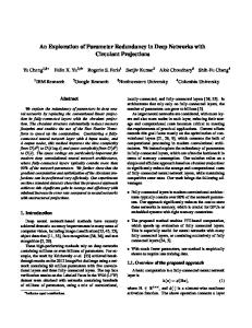
We have constructed a simple scenario to demonstrate all the protocols PDP, DP, MDP-2, MDP-3 and IDP. The network of 15 nodes, numbered from 0 to 14, has been taken to verify the novelty of incorporation controlled redundancy in untrusted environment. The topology of the network is represented in Figure 3.3. We have introduced untrustworthy features in this topology. The increment of misbehaving nodes percentage results in Figure: 3.4, 3.5, 3.6. Introduction of controlled redundancy is achieved through the adaptive approach IDP. We have investigated IDP along with the non-adaptive approaches PDP, DP, MDP-2, MDP-3. For simplicity, we have analyzed all of the algorithms in static environment and considered only deliberate packet drop by intermediate nodes in unsuccessful data transmission. An obvious assumption is that, the source and destination are not among the misbehaving nodes.
Mitigating Misbehavior by Controlled Redundancy
33
0
1
2
Source 10 Destination
5
3
Intermediate 4 9
Misbehaving
8
7
6 13 11
12
14
Figure 3.3: No Misbehaving Node 0
1
2
Source 10 Destination
5
3
Intermediate 4 9
Misbehaving
8
7
6 13 11
12
14
Figure 3.4: Single Misbehaving Node
3.6.2
Simulation
We have calculated the neighbor and two-hop neighbor information from the network topology shown in Table 3.1. We have simulated the broadcast of unicast data packet originated from node 0 and destined to node 14. The other nodes operates as router. We can visualize the creation of forward list when the broadcast packet comes form node 0
Mitigating Misbehavior by Controlled Redundancy
34
0
1
2
Source 10 Destination
5
3
Intermediate 4 9
Misbehaving
8
7
6 13 11
12
14
Figure 3.5: Two Misbehaving Nodes 0
1
2
Source 10 Destination
5
3
Intermediate 4 9
Misbehaving
8
7
6 13 11
12
14
Figure 3.6: Four Misbehaving Nodes to node 2. The nodes in the forward list will involve in further retransmission of the broadcast message. If a node receives duplicate message from different neighbors, it only considers the first one. We have selected the node with minimum identification number to solve the tie.
Mitigating Misbehavior by Controlled Redundancy Non-adaptive Protocols: PDP, DP, MDP-2, MDP-3 • Set of Uncovered Two-hop Neighbor (Uv ): For PDP, Uv = N (N (v)) − N (u) − N (v) − N (N (u) ∩ N (v)) and for all the others, Uv = N (N (v)) − N (u) − N (v) ♦ PDP : U2 =N (N (2)) − N (0) − N (2) − N (N (0) ∩ N (2)) = {0, 1, 2, 3, 6, 7, 8, 9, 10} − {1, 2} − {0, 1, 4, 5} − {3} = {6, 7, 8, 9, 10} ♦ DP, MDP-2, MDP-3 : U2 =N (N (2)) − N (0) − N (2) − N (N (0) ∩ N (2)) = {0, 1, 2, 3, 6, 7, 8, 9, 10} − {1, 2} − {0, 1, 4, 5} = {3, 6, 7, 8, 9, 10} • Set of Possible Retransmitting Nodes (B(u, v)): Table 3.1: Neighbors Within Two Hops v 0 1 2 3 4 5 6 7 8 9 10 11 12 13 14
N (v) 1,2 0,2,3 0,1,4,5 1,4 2,3,6,7,8,9 2,6,7,8,9,10 4,5,11,12 4,5,11 4,5,11,12,13 4,5,12,13 5 6,7,8,14 6,8,9,14 8,9,14 11,12,13
N (N (v)) 1,2,3,4,5 0,2,4,5 0,1,3,6,7,8,9,10 0,2,6,7,8,9 0,1,5,11,12,13 0,1,4,11,12,13 2,3,7,8,9,10,14 2,3,6,8,9,10,14 2,3,6,7,9,10,14 2,3,6,7,8,10,14 2,6,7,8,9 4,5,12,13 4,5,11,13 4,5,11,12 6,7,8,9
35
Mitigating Misbehavior by Controlled Redundancy
36
B(u, v) = N (v) − N (u) Thus, B(0, 2) = N (2) − N (0) ={0, 1, 4, 5} − {1, 2}={4, 5} • Forward list(Fv ): The forward lists are created according to the required number of cover for each of the non-adaptive algorithms. ♦ PDP : Single Cover F2 ={5} ♦ DP : Single Cover F2 ={4,5} ♦ MDP-2 : Double Cover F2 ={4,5} ♦ MDP-3 : Triple Cover F2 ={4,5} Further steps are carried in similar fashion. The detailed steps of the simulation for PDP, DP, MDP-2, MDP-3 are shown in Tables 3.2 and 3.3. Adaptive Protocol: IDP IDP uses the acknowledgement packet received from the destination to identify a successful data transmission. If data packet is not successfully transmitted, then it introduces more redundancy. We can analyze IDP in each of the example networks. • Figure 3.3: No node in the network misbehaves. IDP starts with least redundant protocol, i,e, PDP. As no node misbehaves, the intermediate nodes also rebroadcast the message. Obviously, the data packet will successfully be received by the destination node 14 through 2, 5, 8, 11 and eventually, an acknowledgement packet will be received by sender node 0.
Mitigating Misbehavior by Controlled Redundancy
37
Table 3.2: Simulation of Non-adaptive Broadcasting Protocols : Single Cover u φ 0 0 2 5 8 8
v 0 1 2 5 8 4 11
B(u, v) 1,2 3 4,5 6,7,8,9,10 4,11,12,13 2,3,6,7,9 6,7,14
Uv 3,4,5 φ 6,7,8,9,10 11,12,13 3,14 0,1 φ
Fv 1,2 φ 5 8 4,11 2 φ
(a) PDP
u φ 0 0 1 2 2 4 8
v 0 1 2 3 4 5 8 11
B(u, v) 1,2 3 4,5 4 3,6,7,8,9 6,7,8,9,10 5,11,12,13 6,7,14
Uv 3,4,5 4,5 3,6,7,8,9,10 6,7,8,9 11,12,13 11,12,13 10,14 φ
(b) DP
Fv 1,2 3 4,5 4 8 8 5,11 φ
Mitigating Misbehavior by Controlled Redundancy
38
Table 3.3: Simulation of Non-adaptive Broadcasting Protocols : Multiple Cover u φ 0 0 1 2 2 4 4 4 6 6
v 0 1 2 3 4 5 6 8 9 11 12
B(u, v) 1,2 3 4,5 4 3,6,7,8,9 6,7,8,9,10 5,11,12 5,11,12,13 5,12,13 7,8,14 8,9,14
Uv 3,4,5 4,5 3,6,7,8,9,10 6,7,8,9 11,12,13 11,12,13 10,14 10,14 10,14 13 13
Fv 1,2 3 4,5 4 6,8,9 6,8,9 5,11,12 5,11,12 φ φ φ
(a) MDP-2
u φ 0 0 1 2 2 4 4 4 4 6 6
v 0 1 2 3 4 5 6 7 8 9 11 12
B(u, v) 1,2 3 4,5 4 3,6,7,8,9 6,7,8,9,10 5,11,12 5,11 5,11,12,13 5,12,13 7,8,14 8,9,14
Uv 3,4,5 4,5 3,6,7,8,9,10 6,7,8,9 11,12,13 11,12,13 10,14 10,14 10,14 10,14 13 13
(b) MDP-3
Fv 1,2 3 4,5 4 6,7,8,9 6,7,8,9 5,11,12 5,11 5,11,12 5,11,12 φ φ
Mitigating Misbehavior by Controlled Redundancy
39
• Figure 3.4: Only single node misbehaves, i.e., node 5. IDP first uses the PDP to create the forward list. As it is a misbehaving node, it drops the packet and thus, no acknowledgement packet is received from node 14. The node 4 is not dictated to rebroadcast through any path. Thus, PDP depends solely on node 5 to rebroadcast to convey the message towards 14. After a predefined time, node 0 requests its neighbors to broadcast, but this time with DP. Node 4 and 5 both now rebroadcast. If node 5 does not rebroadcast, then through node 4 we can reach nodes 6, 7, 8, 9 and then to node 14. Thus, the misbehavior of node 5 is alleviated. • Figure 3.5: Two nodes, node 5 and node 8, misbehave. So first two attempts of IDP i.e., the single cover techniques PDP and DP, fall short. IDP then moves to double covering. Both PDP and DP require node 8 to rebroadcast as it is the maximal cover of nodes 11, 12, 13. When node 8 misbehaves, both DP and PDP suffer. But when MDP-2 is used, then nodes 6, 7, 8 are used. The misbehavior of node 8 is thus tackled by nodes 6, 9. • Figure 3.6: The number of misbehaving nodes increases to four. Nodes 5, 6, 8, 9 do not rebroadcast the incoming message. First three attempts of IDP fail. Then the algorithm moves to triple covering using MDP-3. Here node 7 will be requested to rebroadcast to obtain triple covering, and path towards node 14 is achieved through node 7.
3.6.3
Outcome
Analyzing the simulation, we can state that, incorporating the redundancy in a controlled fashion is advantageous to any network which has the probability of presence of any misbehaving node. When there is no misbehaving node, all of the algorithms (PDP, DP, MDP-2, MDP3) successfully transfer the data packet. When a single node, node 5, the least redundant algorithm PDP fails. DP, MDP-2, MDP-3 fail successively when the amount of misbehaving nodes increases in the successive scenarios (Table 3.4). But along with the robustness, we have found the fact that the number of nodes explored increases from PDP to MDP-3 (Table3.5) in all the scenarios, whether it is mandatory or not. For example, it is not required to multicover in Figure 3.3 and PDP is mostly acceptable. But for Figure 3.6, MDP-3 is the best choice. Considering untrustworthiness of the network, another option can be to use solely MDP-2 or
Mitigating Misbehavior by Controlled Redundancy
40
MDP-3 for all the nodes. In this way, reliability can be increased. But, this option adds redundancy to all the nodes in general. Even for the establishment of path with the absence of a single untrusted nodes (see Figure 3.3) it maintains multi cover. This increase in redundancy is only acceptable when there is a pre-conceived notion that the network is highly untrusted one. As percentage of misbehaving nodes in most networks is not so high, applying redundant protocols directly affects the robustness and performance from the perspective of redundancy. Table 3.4: Robustness of Non-adaptive Protocols in Presence of Misbehaving Nodes Misbehaving Nodes None 5 5,8 5,6,8,9
Successful PDP, DP, MDP-2, MDP-3 DP, MDP-2, MDP-3 MDP-2, MDP-3 MDP-3
Table 3.5: Nodes Involved in Broadcasting Algorithm PDP DP MDP-2 MDP-3
Involved Nodes 0,1,2,5,8,11 0,1,2,3,4,5,8,11 0,1,2,3,4,5,6,8,9,11,12 0,1,2,3,4,5,6,7,8,9,11,12
Total Number 6 8 11 12
These shows the applicability of IDP in any untrusted environment. IDP explores the network from least to most whenever an attempt of delivery fails. The number of attempts of IDP is increased in controlled manner with the increment of environment hostility (Table 3.6). Thus IDP ensures reachability in a simple way by taking concern the broadcast storm. Table 3.6: Number of Attempts of IDP Misbehaving Nodes None 5 5,8 5,6,8,9
Number of Attempts 1 2 3 4
Chapter 4 Experimental Results To evaluate the performance of dominant pruning and its variants, we build a detailed simulation model based on NS-2 [1] with wireless extensions. Ns version 2.31 is used for this purpose. The performance of our proposed IDP algorithm was measured along with AODV, DP, MDP-2, MDP-3, PDP and TDP. Before going into the detailed discussion of the simulation result we first define some of the performance metrics.
4.1
Performance Metrics
To see the effect of node misbehavior on variants of dominant pruning and on our proposed enhancements, we consider the following performance metrics• Packet Delivery Fraction (pdf ): Ratio of number of successfully received CBR packets to number of sent CBR packets. If the route discovery of AODV explores the hidden trusted path from source to destination bypassing the misbehaving nodes efficiently, then obviously successful delivery of the data packet will increase. Therefore, the pdf of CBR packet is a useful measure to evaluate the performance of the broadcast. • Routing Overhead : Total number of packets needed to exchange routing information among nodes. • Normalized Routing Load : Fraction of routing packets needed to successfully deliver one data packet. 41
Experimental Results
42
• Average End to End Delay : Average end to end delay is defined as the mean time gap between the initiation of a data packet and the last successful reception of that particular packet. • Average Route Discovery Latency : It is defined as the mean of time taken to find a path between source and destination pairs. • Normalized Efficiency (N.E.): Function of pdf and Routing Overhead defined by the following equation: N.E. =
pdf routingOverhead −c∗ pdfaodv routingOverheadaodv
To scale the reachability measure in respect of redundancy, we propose this new metric, N.E. We incorporate DP and its variants in route discovery process of AODV, which is blind flooding. Thus it is logical to assess the behavior of an approach with respect to pure AODV emphasizing reachability while cutting down redundancy. Here, c is a measure of how routing overhead should be penalized comparing to a successful delivery of data packet. As the size of overhead packet is roughly one tenth of data packet size, 0.1 should be a reasonable assignment for c.
4.2
Scenario Generation
As standard scenario we use a 670m by 670m flat two-dimensional space with 50 nodes. The transmission range of each node is 250m which is roughly
2 5
of each dimension. Pause times of
the nodes are varied from 0 (maximum mobility) to 500 (static scenario) by step size 50. For each such case, 5 random scenarios are generated. Now, a certain percentage of misbehaving nodes is introduced during simulation. These nodes misbehave by dropping packets without rebroadcasting them. The number of misbehaving nodes varies between 0 and 20 with step size 5, which means that the percentage of misbehaving node is from 0% to 40%. As we increase the number of misbehaving nodes, the larger set includes the misbehaving nodes from the previous simulation. This ensures consistency between two scenarios. Similar approaches are mentioned in [18][24].
Experimental Results
4.3
43
Traffic Generation
Traffic sources are CBR (constant bit rate) packets. Total 10 connections are used. Data sources generate unicast packet at regular 1 second intervals. Traffic generators on different sources start at time uniformly distributed between 0 and 50 seconds. The packet size is fixed at 512 bytes. Each simulation runs for 500 seconds of virtual time.
4.4
Novelty of IDP
Table 4.1 shows the percentage of success in different iteration of IDP for the case of route establishment by broadcasting. For example, table 4.2(a) shows that in static scenario and with 0% misbehaving nodes, all the routes are discovered by first two attempts, with PDP and DP. As percentage of misbehaving nodes increases, chances to find routes with these two variants become less probable. With the increase in mobility and misbehaving nodes, success in higher order iterations (MDP-2, 3, infinity) captures greater percentage. These are the cases where traditional approaches of trying with one variant would fail to succeed. Table 4.1 also stands for the redundancy control of IDP, because for all cases, least redundant version PDP (1st iteration) takes a major portion of obtaining success.
4.5
Graphical Comparison
4.5.1
Constant Pause Time
• Packet Delivery Fraction (pdf ): Figure 4.1 illustrates the effect of node misbehavior on pdf observed for various approaches. For a static scenario (Fig:4.1(a)), versions with sufficient redundancy (AODV, MDP 2, MDP 3, IDP) make clusters and show high degree of reachability even with a considerable number of misbehaving nodes. Other techniques (PDP, TDP, DP) suffer a lot in the presence of misbehaving nodes and their performance degrades considerably. With the increase in mobility (Fig: 4.1(b), 4.1(c)) AODV performs the best, but still performance of IDP is very close to other redundant ones. • Normalized Efficiency (N.E.): Figure 4.2 shows the effect of node misbehavior on
Experimental Results
44
Table 4.1: Distribution of Successful route-setup in iterations of IDP
Percentage of Misbehaving Nodes Iteration 0% 1st 2nd 3rd 4th 5th
10%
20%
30%
40%
95.00% 80.00% 70.83% 57.14% 56.53% 5.00% 12.00% 12.50% 17.86% 13.04% 0% 4.00% 12.50% 21.43% 26.08% 0% 4.00% 4.17% 3.57% 4.35% 0% 0% 0% 0% 0% (a) Static Environment, Pause Time: 500
Percentage of Misbehaving Nodes Iteration 1st 2nd 3rd 4th 5th
0%
10%
88.24% 8.09% 2.94% 0% 0.74%
89.23% 6.15% 4.62% 0% 0%
20%
30%
40%
83.70% 78.81% 68.67% 7.41% 10.17% 12.00% 6.67% 6.78% 10.67% 1.48% 2.55% 6.00% 0.74% 1.69% 2.66%
(b) Average Mobility, Pause Time: 250
Percentage of Misbehaving Nodes Iteration 1st 2nd 3rd 4th 5th
0%
10%
91.94% 4.03% 3.66% 0.37% 0%
90.68% 5.73% 2.51% 0.72% 0.36%
20%
30%
40%
88.73% 83.57% 83.86% 5.88% 7.25% 4.93% 3.92% 6.28% 6.28% 1.47% 1.93% 3.14% 0% 0.97% 1.79%
(c) Highest Mobility, Pause Time: 0
Experimental Results
45
N.E. In static scenario, performance of IDP lies above of most other variants. Not surprisingly, in mobile situations IDP is a clear winner. Though, with respect to successful delivery IDP may not be the best, its routing overhead is as low as other less redundant versions like TDP, PDP, DP. That is why N.E is observed to be the best in IDP. • Normalized Routing Load : In mobile scenario (Fig: 4.3(b), 4.3(c)), IDP is one of the best along with DP, the least redundant version. The normalized routing load remains much more constant with the increment of percentage of malicious nodes. • Average End to End Delay : In Figure 4.4, AODV is the best as it incorporates blind flooding. IDP introducing controlled redundancy thus ensures reachability with some degradation in Average End to End Delay. The delay increases with environment hostility. • Average Route Discovery Latency : In static(Fig: 4.5(a) and moderately mobile(Fig: 4.5(b)) environment, IDP is very close to other versions. In highly mobile scenario(Fig: 4.5(c)), it is higher than AODV but remains very close to other versions(DP, MDP-2, MDP-3) and remains approximately constant in varying percentage of malicious nodes.
4.5.2
Constant Percentage of Malicious Nodes
• Packet Delivery Fraction (pdf ):For totally trustworthy environment(Fig: 4.6(a)), pdfs of all the versions are very close and increase with the increment of mobility. In more hostile environment(Fig: 4.6(b), 4.6(c)), pdf of IDP shows minute increment along with the other versions, as environment hostility is mitigated by the mobility of nonmalicious nodes, which ensures successful packet delivery. • Normalized Efficiency (N.E.): Figure 4.7 shows the effect of mobility on N.E. In all the cases, redundant approaches are almost oblivious to mobility and does not suffer much even in the presence of 40% misbehaving nodes. Performance of less redundant variants degrades largely in lower mobility, as unreachable destinations remain unreachable most of the times.
Experimental Results
46
• Normalized Routing Load :Figure 4.8 shows that TDP and PDP incur the lowest amount of redundancy, as expected. IDP is also very close to these two and does not change much with the change in percentage of misbehaving nodes. • Average End to End Delay : It decreases as mobility increases in all the scenarios(Figure: 4.9). The graph of IDP is clustered with that of DP but has minute difference with others(AODV, MDP-2, MDP-3). • Average Route Discovery Latency : Route Discovery Latencies of all the versions remain mostly constant throughout each graph (Figure: 4.10). We can realize the fact that, Route Discovery Latency is unaffected by host mobility.
Experimental Results
47
1
Packet Delivery Fraction
0.95 0.9 0.85 0.8 AODV IDP MDP 3 MDP 2 DP PDP TDP
0.75 0.7 0.65 0
10 20 30 Percentage of Misbehaving Nodes
40
(a) Static Environment, Pause Time: 500
1
Packet Delivery Fraction
0.98 0.96 0.94 0.92 0.9
AODV IDP MDP 3 MDP 2 DP PDP TDP
0.88 0.86 0.84 0
10 20 30 Percentage of Misbehaving Nodes
40
(b) Average Mobility, Pause Time: 250
0.99
Packet Delivery Fraction
0.98 0.97 0.96 0.95 AODV IDP MDP 3 MDP 2 DP PDP TDP
0.94 0.93 0.92 0
10 20 30 Percentage of Misbehaving Nodes
40
(c) Highest Mobility, Pause Time: 0
Figure 4.1: Packet Delivery Fraction with Varying Percentage of Misbehaving Node
Experimental Results
48
0.95
Normalized Efficiency
0.9 0.85 0.8 0.75 AODV IDP MDP 3 MDP 2 DP PDP TDP
0.7 0.65 0.6 0
10 20 30 Percentage of Misbehaving Nodes
40
(a) Static Environment, Pause Time: 500
0.96
Normalized Efficiency
0.94 0.92 0.9 0.88 0.86 AODV IDP MDP 3 MDP 2 DP PDP TDP
0.84 0.82 0.8 0.78 0
10 20 30 Percentage of Misbehaving Nodes
40
(b) Average Mobility, Pause Time: 250
0.97
Normalized Efficiency
0.96 0.95 0.94 0.93 AODV IDP MDP 3 MDP 2 DP PDP TDP
0.92 0.91 0.9 0
10 20 30 Percentage of Misbehaving Nodes
40
(c) Highest Mobility, Pause Time: 0
Figure 4.2: Normalized Efficiency with Varying Percentage of Misbehaving Node
Experimental Results
49
0.5
AODV IDP MDP 3 MDP 2 DP PDP TDP
Normalized Routing Load
0.45 0.4 0.35 0.3 0.25 0.2 0.15 0.1 0
10 20 30 Percentage of Misbehaving Nodes
40
(a) Static Environment, Pause Time: 500
0.7
AODV IDP MDP 3 MDP 2 DP PDP TDP
Normalized Routing Load
0.65 0.6 0.55 0.5 0.45 0.4 0.35 0.3 0.25 0
10 20 30 Percentage of Misbehaving Nodes
40
(b) Average Mobility, Pause Time: 250
1.6
AODV IDP MDP 3 MDP 2 DP PDP TDP
Normalized Routing Load
1.4 1.2 1 0.8 0.6 0.4 0.2 0
10 20 30 Percentage of Misbehaving Nodes
40
(c) Highest Mobility, Pause Time: 0
Figure 4.3: Normalized Routing Load with Varying Percentage of Misbehaving Node
Experimental Results
50
0.065
AODV IDP MDP 3 MDP 2 DP PDP TDP
Avg End to End Delay
0.06 0.055 0.05 0.045 0.04 0.035 0.03 0.025 0.02 0
10 20 30 Percentage of Misbehaving Nodes
40
(a) Static Environment, Pause Time: 500
0.25
AODV IDP MDP 3 MDP 2 DP PDP TDP
Avg End to End Delay
0.2
0.15
0.1
0.05
0 0
10 20 30 Percentage of Misbehaving Nodes
40
(b) Average Mobility, Pause Time: 250
0.35
AODV IDP MDP 3 MDP 2 DP PDP TDP
Avg End to End Delay
0.3 0.25 0.2 0.15 0.1 0.05 0 0
10 20 30 Percentage of Misbehaving Nodes
40
(c) Highest Mobility, Pause Time: 0
Figure 4.4: Average End to End Delay with Varying Percentage of Misbehaving Node
Experimental Results
51
12
AODV IDP MDP 3 MDP 2 DP PDP TDP
Route Discovery Latency
10 8 6 4 2 0 0
10 20 30 Percentage of Misbehaving Nodes
40
(a) Static Environment, Pause Time: 500
35
AODV IDP MDP 3 MDP 2 DP PDP TDP
Route Discovery Latency
30 25 20 15 10 5 0 0
10 20 30 Percentage of Misbehaving Nodes
40
(b) Average Mobility, Pause Time: 250
3.5
AODV IDP MDP 3 MDP 2 DP PDP TDP
Route Discovery Latency
3 2.5 2 1.5 1 0.5 0 0
10 20 30 Percentage of Misbehaving Nodes
40
(c) Highest Mobility, Pause Time: 0
Figure 4.5: Average Route Discovery Latency with Varying Percentage of Misbehaving Node
Experimental Results
52
1
Packet Delivery Fraction
0.995 0.99 0.985 0.98 0.975
AODV IDP MDP 3 MDP 2 DP PDP TDP
0.97 0.965 0.96 0
50
100
150
200 250 300 Pause Time
350
400
450
500
350
400
450
500
350
400
450
500
(a) 0% Misbehaving Node
1
Packet Delivery Fraction
0.98 0.96 0.94 0.92 0.9
AODV IDP MDP 3 MDP 2 DP PDP TDP
0.88 0.86 0.84 0
50
100
150
200 250 300 Pause Time
(b) 20% Misbehaving Node
1
Packet Delivery Fraction
0.95 0.9 0.85 0.8 AODV IDP MDP 3 MDP 2 DP PDP TDP
0.75 0.7 0.65 0
50
100
150
200 250 300 Pause Time
(c) 40% Misbehaving Node
Figure 4.6: Packet Delivery Fraction with Varying Pause Time
Experimental Results
53
0.98
Normalized Efficiency
0.96 0.94 0.92 0.9 AODV IDP MDP 3 MDP 2 DP PDP TDP
0.88 0.86 0.84 0
50
100
150
200 250 300 Pause Time
350
400
450
500
350
400
450
500
350
400
450
500
(a) 0% Misbehaving Node
1
Normalized Efficiency
0.95 0.9 0.85 AODV IDP MDP 3 MDP 2 DP PDP TDP
0.8 0.75 0.7 0
50
100
150
200 250 300 Pause Time
(b) 20% Misbehaving Node
0.95
Normalized Efficiency
0.9 0.85 0.8 0.75 AODV IDP MDP 3 MDP 2 DP PDP TDP
0.7 0.65 0.6 0
50
100
150
200 250 300 Pause Time
(c) 40% Misbehaving Node
Figure 4.7: Normalized Efficiency with Varying Pause Time
Experimental Results
54
1.6
AODV IDP MDP 3 MDP 2 DP PDP TDP
Normalized Routing Load
1.4 1.2 1 0.8 0.6 0.4 0.2 0 0
50
100
150
200 250 300 Pause Time
350
400
450
500
450
500
450
500
(a) 0% Misbehaving Node
1.2
AODV IDP MDP 3 MDP 2 DP PDP TDP
Normalized Routing Load
1 0.8 0.6 0.4 0.2 0 0
50
100
150
200 250 300 Pause Time
350
400
(b) 20% Misbehaving Node
0.9
AODV IDP MDP 3 MDP 2 DP PDP TDP
Normalized Routing Load
0.8 0.7 0.6 0.5 0.4 0.3 0.2 0.1 0
50
100
150
200 250 300 Pause Time
350
400
(c) 40% Misbehaving Node
Figure 4.8: Normalized Routing Load with Varying Pause Time
Experimental Results
55
0.14
AODV IDP MDP 3 MDP 2 DP PDP TDP
Avg End to End Delay
0.12 0.1 0.08 0.06 0.04 0.02 0 0
50
100
150
200 250 300 Pause Time
350
400
450
500
450
500
450
500
(a) 0% Misbehaving Node
0.22
AODV IDP MDP 3 MDP 2 DP PDP TDP
0.2
Avg End to End Delay
0.18 0.16 0.14 0.12 0.1 0.08 0.06 0.04 0.02 0 0
50
100
150
200 250 300 Pause Time
350
400
(b) 20% Misbehaving Node
0.5
AODV IDP MDP 3 MDP 2 DP PDP TDP
0.45
Avg End to End Delay
0.4 0.35 0.3 0.25 0.2 0.15 0.1 0.05 0 0
50
100
150
200 250 300 Pause Time
350
400
(c) 40% Misbehaving Node
Figure 4.9: Average End to End Delay with Varying Pause Time
Experimental Results
56
8
AODV IDP MDP 3 MDP 2 DP PDP TDP
Route Discovery Latency
7 6 5 4 3 2 1 0 0
50
100
150
200 250 300 Pause Time
350
400
450
500
350
400
450
500
400
450
500
(a) 0% Misbehaving Node
16
AODV IDP MDP 3 MDP 2 DP PDP TDP
Route Discovery Latency
14 12 10 8 6 4 2 0 0
50
100
150
200 250 300 Pause Time
(b) 20% Misbehaving Node
50
AODV IDP MDP 3 MDP 2 DP PDP TDP
Route Discovery Latency
45 40 35 30 25 20 15 10 5 0 0
50
100
150
200 250 300 Pause Time
350
(c) 40% Misbehaving Node
Figure 4.10: Average Route Discovery Latency with Varying Pause Time
Chapter 5 Conclusion and Future Work 5.1
Summary
This dissertation considers several problems regarding broadcast in untrusted ad hoc wireless network. At first, we have presented issues that require attentive consideration in designing an efficient broadcast algorithm. A categorization of broadcast algorithm have been discussed. The categorization depends on the exploitation of local neighborhood information. In fact, in ad hoc network, local neighborhood information is easy for nodes to collect and disseminate as no central infrastructure is there to control communication. From the discussions throughout the dissertation and simulation results, it is clear that least redundant protocol like PDP, TDP, DP suffer badly in the presence of untrusted nodes. Adding redundancy with MDP can be a remedy but that redundancy is not desirable in the cooperative trusted environment. As in the general case percentage of misbehaving nodes is not so high, blind deployment of MDP with m >= 2 is not effective from the perspective of network traffic. These issues demand a technique that lies somewhere in the middle of the above two. Our presented idea, IDP finds a dynamic way that cuts down redundancy for normal cases and incorporates controlled amount of redundancy only for the paths where any misbehaving nodes might be present. We can say that, though redundancy is undesired in trusted environment, controlled redundancy is effective for ad hoc networks where no assumption can be made about operational environment. This concluding remark is justified greatly in our simulation results. IDP has similar reachability as pure AODV which is the same as blind flooding and at the
57
Conclusion and Future Work
58
same time has lower overhead as that of PDP and TDP. Therefore, it is desirable from both aspects. This approach will perform very well in trusted environment, though it is designed to be used in untrusted ones. This is because, when no misbehaving node is present, this algorithm will choose the least possible value of m and thus ensure lowest redundancy.
5.2
Future Work
We plan to investigate the effect of tuning the redundancy parameter m in some distinct scenarios. One assumption we adopt in favor of incrementing m is that - most of the packet drops are due to route disassociation, not due to broadcast storm. But in latter cases, we can tune m to be decremented whenever packet drop is due to collision or congestion and increment otherwise. As our simulations were done with CBR packets, no reliability requirements were taken. Our next goal is to analyze how our proposed algorithm performs with TCP, which is common to most network applications.
Appendix
NS2, The Network Simulator
NS2 The Network Simulator ●
What is NS-2
●
Installation
●
Set Path
●
Validation
●
Scenario Generation
●
CBR Traffic Generation
●
Generate Simulation
●
Trace Generation
●
Trace Analysis
●
Links
●
Contact Us
What is NS-2 ●
NS is an object-oriented,discrete event simulator targeted at networking research. Ns provides substantial support for simulation of TCP, routing, and multicast protocols over wired and wireless (local and satellite) networks. Later NS-2 (version 2) was developed at UC Berkeley in C++ and OTcl (Object-oriented extension of Tcl)
Installation ● ● ●
●
Download NS2 version 2.31 from here Unzip the tar archive Open Terminal and Go to the ns2 root directory. Here ~/ns-allinone-2.31 Run ./install script
Set Path ●
●
●
After installation to set the path type the following contents ❍ Export LD_LIBRARY_PATH=~ns-allinone2.31/otcl-1.13 ❍ Export LD_LIBRARY_PATH=~ns-allinone2.31/ns-2.31/lib ❍ Export TCL_LIBRARY=~ns-allinone-2.31/ tcl8.4.14/library To access ns command in any directory ❍ Go to ns2.31 directory under the ns-allinone2.31 ❍ Execute the command make install To access setdest command in any directory ❍ Go to ns2.31/indep-utils/cmu-scen-gen/ setdest directory under the ns-allinone-2.31 ❍ Execute the command make install
Validation ● ● ●
Open terminal in ~ns-allinone-2.31/ns-2.31 Run ./validate If installation and path variable setting are done properly, then the validation will be successful
Scenario Generation
http://teacher.buet.ac.bd/ashikur/ns2/ (1 of 4)3/6/2009 12:36:20 AM
NS2, The Network Simulator
●
●
●
●
●
This is done using the setdest command. There are two versions for setdest. Version 2 is most recently implemented and used. Version 2 signature of setdest command is setdest -v <2> -n
-s m -M -t -P -p -x -y ❍ -v version number; Here 2 ❍ -n number of nodes. Generated node number will be 0 to (n-1) ❍ -s speed type (uniform, normal); s=1 uniform speed from min to max; s=2 normal speed clipped from min to max ❍ -m minimum speed > 0 ❍ -M maximum speed ❍ -P pause type (constant, uniform); P=1 constant pause; P=2 uniform pause [0, 2*p] ❍ -p pause time (a median if uniform is chosen) ❍ -x x dimension of space ❍ -y y dimension of space After running the command a scenario will be generated. Pipe the scenario in file Example ❍ setdest -v 2 -n 10 -m 10 -M 100 -t 20 -P 1 p 10 -x 200 -y 400 > scen-exp1 For Further Explanation: Go through the source code ~ns-allinone-2.31/ns-2.31/indep-utils/ cmu-scen-gen/setdest/setdest.cc
CBR Traffic Generation ●
●
●
●
●
●
http://teacher.buet.ac.bd/ashikur/ns2/ (2 of 4)3/6/2009 12:36:20 AM
This is done with the help of cbrgen.tcl file executing with ns command Open terminal in ~ns-allinone-2.31/ns-2.31/indeputils/cmu-scen-gen ns cbrgen.tcl [-type cbr|tcp] [-nn nodes] [seed seed] [-mc connections] [-rate rate] ❍ -type traffic type (tcp, udp/cbr) ❍ -nn the highest node number(node number will be 0 to nn) ❍ -seed seed for random variable generation which is used to create random number of source-destination pair ❍ -mc maximum number of connections; i.e.; source-destination pair ❍ -rate it is the inverse of the interval between packet transmission & should be <0 After running the command a cbr traffic will be generated. Pipe the traffic in file Example ❍ ns cbrgen.tcl -type cbr -nn 9 -seed 1 -mc 10 -rate .25 > cbr-exp1 For Further Explanation: Go through the source
NS2, The Network Simulator
code ~ns-allinone-2.31/ns-2.31/indep-utils/ cmu-scen-gen/cbrgen.tcl
Writing Simulation Generation File ●
●
●
http://teacher.buet.ac.bd/ashikur/ns2/ (3 of 4)3/6/2009 12:36:20 AM
Download this sample tcl file or write a new tcl file. This sample should give some idea of the different parameters that need to be configured for a typical simulation. A wireless simulation is made up of some number of MobileNodes. Each such mobile node needs some options to be configured like routing protocol, MAC layer protocol, antenna type, channel type etc. A list of all parameters is given below. ❍ Channel type (Channel/ WirelessChannel) ;# Set channel for wireless media ❍ Propagation model (Propagation/ TwoRayGround); ❍ Interface type (Phy/WirelessPhy) ; ❍ MAC layer protocol (Mac/802_11) ;# The name of MAC layer protocol ❍ Routing protocol (AODV) ;# The name of routing protocol ❍ Interface Queue type (CMUPriQueue for DSR) ; ❍ Interface Queue Length (50) ;# Queue length of a node for storing packets ❍ Antenna type (Antenna/ OmniAntenna) ;# ❍ LL type (LL) ;# Link Layer type Set the required parameters in the tcl file for the specific scenario and traffic. These are the configuration parameters for the topology structure, like the dimensions of the grid, number of nodes present etc. A list of all of them is given below for reference. Example(For the previous scenario and traffic) ❍ set val(x) 200 ;# X dimension of the topography ❍ set val(y) 400 ;# Y dimension of the topography ❍ set val(ifqlen) 50 ;# max packet in ifq ❍ set val(seed) 0.0 ; ❍ set val(adhocRouting) AODV ;# The routing protocol ❍ set val(nn) 10 ;# how many nodes are simulated ❍ set val(cp) "cbr-exp1" ;# the absolute or relative path of the traffic file ❍ set val(sc) "scen-exp1" ;# the absolute or relative path of the scenario file ❍ set val(stop) 200.0 ;# the simulation time Turn on the trace for the required layers Example ❍ -agentTrace ON \
NS2, The Network Simulator
-routerTrace ON \ ❍ -macTrace ON \ ❍ -movementTrace OFF For generating the trace file in new format, remove the comment or vice versa $ns_ use-newtrace Set the output trace file with absolute or relative path Example: set tracefd [open exp1.tr w] ❍
●
●
Trace Generation ●
●
●
●
●
http://teacher.buet.ac.bd/ashikur/ns2/ (4 of 4)3/6/2009 12:36:20 AM
Paste the tcl file to the ~ns-allinone-2.31/ns2.31/tcl/ex directory Open terminal in ~ns-allinone-2.31/ns-2.31/ tcl/ex Execute commandns Example: ns sample.tcl If the simulation is successful, the desired trace file will be generated. Click here for a sample tcl file for wireless simulation.
NS2, The Network Simulator
NS2 The Network Simulator ●
Back to Home
●
Links
●
Trace Analysis
●
Contact Us
Trace Analysis The various traces begin with a single character or abbreviation that indicates the type of trace, followed by a fixed or variable trace format. Example of new wireless trace format is ●
●
s -t 163.001503520 -Hs 0 -Hd -2 -Ni 0 -Nx 300.00 -Ny 500.00 -Nz 0.00 -Ne -1.000000 -Nl AGT -Nw --- -Ma 0 -Md 0 -Ms 0 -Mt 0 -Is 0.0 Id 2.0 -It cbr -Il 200 -If 1 -Ii 77 -Iv 32 -Pn cbr Pi 32 -Pf 0 -Po 0 ;
Illustration of various fields : Field 0: Event type : Event type (as in the older trace format) In the traces above, describes the type of event taking place at the node and can be one of the four types ❍ ❍ ❍ ❍
●
Field 1: General Tag : The second field starting with "-t" may stand for time ❍
●
● ●
●
s: send r: receive d: drop f: forward
-t : time
Field 3: Next hop info -Hs: id for this node -Hd: id for next hop towards the destination
Field 4: Node property type tag :
http://teacher.buet.ac.bd/ashikur/ns2/traceanalysis.html (1 of 3)3/6/2009 12:36:52 AM
NS2, The Network Simulator
This field denotes the node properties like nodeid, the level at which tracing is being done like agent, router or MAC. The tags start with a leading "-N" and are listed as below: ● ● ● ● ●
-Ni: node id -Nx –Ny -Nz: node’s x/y/z coordinate -Ne: node energy level -Nl: trace level, such as AGT, RTR, MAC -Nw: reason for the event .The different reasons
for dropping a packet are given below: "END" DROP_END_OF_SIMULATION "COL" DROP_MAC_COLLISION "DUP" DROP_MAC_DUPLICATE "ERR" DROP_MAC_PACKET_ERROR "RET" DROP_MAC_RETRY_COUNT_EXCEEDED "STA" DROP_MAC_INVALID_STATE "BSY" DROP_MAC_BUSY131 "NRTE" DROP_RTR_NO_ROUTE i.e no route is available. "LOOP" DROP_RTR_ROUTE_LOOP i.e there is a routing loop "TTL" DROP_RTR_TTL i.e TTL has reached zero. "TOUT" DROP_RTR_QTIMEOUT i.e packet has expired. "CBK" DROP_RTR_MAC_CALLBACK "IFQ" DROP_IFQ_QFULL i.e no buffer space in IFQ. "ARP" DROP_IFQ_ARP_FULL i.e dropped by ARP "OUT" DROP_OUTSIDE_SUBNET i.e i. e dropped by base stations on receiving routing updates from nodes outside its domain.
●
● ● ●
Field 5: Packet information at IP level : The tags for this field start with a leading "-I" and are listed along with their explanations as following: -Is: source address. Source port number -Id: destination address.destination port number -It: packet type
http://teacher.buet.ac.bd/ashikur/ns2/traceanalysis.html (2 of 3)3/6/2009 12:36:52 AM
NS2, The Network Simulator ● ● ● ●
●
-Il: packet size -If: flow id -Ii: unique id -Iv: ttl value
Field 6: Packet information at MAC level : This field gives MAC layer information and starts with a leading "-M" as shown below
●
-Ma: duration -Md: destination’s ethernet address -Ms: source’s ethernet address -Mt: ethernet type
●
Field 7: Packet info at “Application level” :
● ● ●
The packet information at the application level consists of the type of application like arp, tcp, the type of adhoc routing protocol like DSDV, DSR, AODV etc. The field consists of a leading – P and the list of tags for different applications. For example with TCP protocol. ●
● ● ●
-P tcp: Information about TCP flow is given by the following subtags. -Ps: seq number -Pf: how many times this pkt was forwarded -Po: optimal number of forwards
http://teacher.buet.ac.bd/ashikur/ns2/traceanalysis.html (3 of 3)3/6/2009 12:36:52 AM
NS2, The Network Simulator
NS2 The Network Simulator ●
Back to Home
●
Trace Analysis
●
Links
●
Links for NS-2 related websites and mailing lists ●
Contact Us ●
●
●
● ● ●
NS official Website : http://www.isi.edu/ nsnam/ns Tutorial : http://www.isi.edu/nsnam/ns/ tutorial/ Documentation : http://www.isi.edu/nsnam/ ns/ns-documentation.html Mailing list : http://mailman.isi.edu/mailman/ listinfo/ns-users http://nile.wpi.edu/NS/ http://evanjones.ca/ns2.html http://sourceforge.net/projects/nsnam/
http://teacher.buet.ac.bd/ashikur/ns2/links.html3/6/2009 12:37:38 AM
NS2, The Network Simulator
The Network Simulator ●
Back to Home
●
links
●
Trace Analysis
●
Contact us
Motivation ●
This site is developed and maintained by Nashid Shahriar, Arup Raton Roy, Syed Ashker Ibne Mujib, students of the thesis group under Dr. A.K.M Ashikur Rahman, Assistant professor, Bangladesh University of Engineering & Technology. Our thesis topic is "Effect of Redundancy on Broadcasting in Untrusted Ad hoc Wireless Network". We are working on AODV and our supporting simulator is NS-2, a very useful tool for networking related works. Initially we felt the necessity of a tutorial website for wireless version of NS-2 when becoming familiar with it. From that realization we gather our experiences and observations in this site.
Contact us ●
This site is for the beginners who are becoming familiar with wireless networking in NS-2. If you have any query or need help or have found any kind of discrepancy in the information provided here please let us know. Also feel free to share your thoughts and suggestions about the website at [email protected] .
http://teacher.buet.ac.bd/ashikur/ns2/contact.html3/6/2009 12:37:54 AM
Bibliography [1] The Network Simulator: NS-2: notes and documentation. http://www.isi.edu/nsnam/ns/. [2] K. M. Alzoubi, P. J. Wan and O. Frieder. New distributed algorithm for connected dominating set in wireless ad hoc networks.
In Proc. HICSS-35, 2002.
[3] J. Broch, D. A. Maltz, D. B. Johnson, Y. C. Hu and J. Jetcheva. A performance comparison of multi-hop wireless ad hoc network routing protocols. In Proc. IEEE/ACM Intl. Conf. on Mobile Computing and Networking MOBICOM, pages 85-97, 1998 [4] G. Calinescu, I. Mandoiu, P. J. Wan and A. Zelikovsky. Selecting forwarding neighbors in wireless ad hoc networks. In Proc. ACM DIALM’2001, pp. 34-43, Dec. 2001. [5] J. Cartigny and D. Simplot. Border node retransmission based probabilistic broadcast protocols in ad-hoc networks.
In Proceedings Hawaii International Conference on System
Sciences (HICSS-36), 2003. [6] T. H. Corman, C. E. Leiserson, R. L. Rivest, and C. Stein. Introduction to Algorithm. MIT Press, Cambridge, MA, USA, 2001. [7] B. Das, R. Sivakumar, and V. Bharghavan. Routing in ad-hoc networks using a virtual backbone.
In Proceedings International Conference on Computer Communications and
Networks (ICCCN), pages 120, 1997. [8] M. Gerla and J. T. Tsai. Multicluster, mobile, multimedia radio network.
In Proceedings
of ACM-Baltzer Journal of Wireless Networks, pages 255265, 1995. [9] Z. J. Haas, J. Y. Halpern, and L. Li. Gossip-based ad hoc routing. INFOCOM, pages 17071716, 2002. 68
In Proceedings
Bibliography
69
[10] Z. J. Haas and M. R. Pearlman. The zone routing protocol (ZRP) for ad hoc networks. 1998, Internet Draft. [11] M.E. Hoque, F. Rahman, S. K. Kundu, A. Rahman, and P. Gburzynski, Enhanced Partial Dominant Pruning (EPDP) Based Broadcasting in Ad hoc Wireless Networks.
In
Proceedings of SPECTS 2008, Edinburgh, UK, June 2008. [12] M. Jiang, J. Li and Y. C. Tay. Cluster based routing protocol (CBRP) functional specification. 1998, Internet Draft. [13] D. B. Johnson and D. A. Maltz. Dyanmic Source Routing in ad hoc wireless networks. In Imielinski and Korth, editors, Mobile Computing, volume 353, Kluwer Academic Publishers, 1996 [14] Y. Ko and N. H. Vaidya. Location-aided routing (LAR) in mobile ad hoc networks.
In
Proceedings of the ACM/IEEE International Conference on Mobile Computing and Networking (MOBICOM), pages 6675, 1998. [15] D. Lichtenstein. Planar formulae and their uses.
In SIAM Journal on Computing, 11(2):
329-343, 1982 [16] H. Lim and C. Kim. Multicast tree construction and flooding in wireless ad hoc networks. In ACM International Workshop on Modeling, Analysis and Simulation of Wireless and Mobile Systems (MSWIM), 2000. [17] W. Lou and J. Wu. On reducing broadcast redundancy in ad-hoc wireless networks.
In
IEEE Transactions on Mobile Computing, 1(2): 111-123, 2002. [18] S. Marti, T. J. Giuli, Kevin Lai and M. Baker. Mitigating routing misbehavior in mobile ad hoc networks. In Mobile Computing and Networking, pages 255-265, 2000. [19] A. Mishra. Security and Quality of Service in Ad hoc Wireless Networks.
Cambridge
University Press, Cambridge, UK, 2008. [20] S. Ni, Y. Tseng, Y. Chen and J. Sheu. The broadcast storm problem in a mobile ad hoc network. In Proc. Mobicom’99, pp. 151-162, Aug. 1999.
Bibliography
70
[21] W. Peng and X. C. Lu. On the reduction of broadcast redundancy in mobile ad hoc networks. In Proc. First Annual Workshop on Mobile and Ad Hoc Networking and Computing, MOBIHOC, pp. 129-130, Aug. 2000, Boston, USA. [22] C. E. Perkins, E. M. Royers and S. R. Das. Ad-hoc On-demand Distance Vector Routing (AODV), February 2003. Internet Draft: draft-ietf-manet-aodv-13.txt. [23] A. Qayyum, L. Viennot and A. Laouiti. Multipoint relaying for flooding broadcast message in mobile wireless networks. In Proc. HICSS-35, Jan. 2002. [24] A. Rahman, P. Gburzynski and B. Kaminska. Enhanced Dominant Pruning-based Broadcasting in Untrusted Ad-hoc Wireless Networks. In ICC, 2007. [25] E. M. Royer and C. K. Toh. A review of current routing protocols for ad hoc mobile wireless networks. In IEEE Personal Communications,, 6(2):46-55, 1999. [26] J. Wu and F. Dai. Broadcasting in ad hoc networks based on self-pruning. INFOCOM, March 2003.
In Proc. of