On Approximation Resistance of Predicates
Algorithm Hardness
Subhash Khot New York University
zero-sum game
Joint work with Madhur Tulsiani and Pratik Worah
value = 0 ?
Overview of the Talk
- Introduction and Survey - Basics: Algorithmic Side - Basics: Hardness Side - Characterization of Approximation Resistance - Conclusion
Constraint Satisfaction Problems (CSP)
Constraint Satisfaction Problems (CSP) - Boolean ({−1, 1}-valued) variables and constraints.
Constraint Satisfaction Problems (CSP) - Boolean ({−1, 1}-valued) variables and constraints. - All constraints of same type, variable negation allowed.
3-SAT x1 ∨ x22 ∨ x 19 x3 ∨ x 9 ∨ x23 x5 ∨ x 7 ∨ x 9 .. .
Constraint Satisfaction Problems (CSP) - Boolean ({−1, 1}-valued) variables and constraints. - All constraints of same type, variable negation allowed.
3-SAT
CUT x1
x1 ∨ x22 ∨ x 19
x2
x3 ∨ x 9 ∨ x23 x5 ∨ x 7 ∨ x 9 .. .
x4 x5
x7 x6
x3
Constraint Satisfaction Problems (CSP) - Boolean ({−1, 1}-valued) variables and constraints. - All constraints of same type, variable negation allowed.
3-SAT
CUT x1
x1 ∨ x22 ∨ x 19
x2
x3 ∨ x 9 ∨ x23 x5 ∨ x 7 ∨ x 9 .. .
x4 x5
x7 x6
x3
x1 = 6 x2 x2 = 6 x5 x3 = 6 x4 .. .
Constraint Satisfaction Problems (CSP) 3-XOR: Linear equations modulo 2 (in ±1 variables)
Constraint Satisfaction Problems (CSP) 3-XOR: Linear equations modulo 2 (in ±1 variables) x5 · x9 · x16 = 1 x6 · x12 · x22 = −1 x7 · x8 · x15 = −1 .. .
Constraint Satisfaction Problems (CSP) 3-XOR: Linear equations modulo 2 (in ±1 variables) x5 · x9 · x16 = 1
x5 · x9 · x16 = 1
x6 · x12 · x22 = −1
x6 · x 12 · x22 = 1
x7 · x8 · x15 = −1 .. .
−→
x7 · x8 · x 15 = 1 .. .
Constraint Satisfaction Problems (CSP) 3-XOR: Linear equations modulo 2 (in ±1 variables) x5 · x9 · x16 = 1
x5 · x9 · x16 = 1
x6 · x12 · x22 = −1
x6 · x 12 · x22 = 1
x7 · x8 · x15 = −1 .. .
−→
x7 · x8 · x 15 = 1 .. .
CSP(f ) : Given predicate f : {−1, 1}k → {0, 1}. Each constraint is f applied to some k (possibly negated) variables.
Constraint Satisfaction Problems (CSP) 3-XOR: Linear equations modulo 2 (in ±1 variables) x5 · x9 · x16 = 1
x5 · x9 · x16 = 1
x6 · x12 · x22 = −1
x6 · x 12 · x22 = 1
x7 · x8 · x15 = −1 .. .
−→
x7 · x8 · x 15 = 1 .. .
CSP(f ) : Given predicate f : {−1, 1}k → {0, 1}. Each constraint is f applied to some k (possibly negated) variables. C ≡ f xi1 , x i2 , . . . , x ik−1 , xik
�
k fixed constant. Number of variables and constraints → ∞.
Constraint Satisfaction Problems (CSP) x1 x2
x4
x5
x7
x3
x6 CSP(f ) : Given predicate f : {−1, 1}k → {0, 1}. Each constraint is f applied to some k (possibly negated) variables. C ≡ f xi1 , x i2 , . . . , x ik−1 , xik
�
k fixed constant. Number of variables and constraints → ∞.
Satisfiability vs Approximability
- [Schaefer 78], Dichotomy Theorem: For every predicate f : {−1, 1}k → {0, 1}, deciding the satisfiability of CSP(f ) is either in P or is NP-hard.
Satisfiability vs Approximability
- [Schaefer 78], Dichotomy Theorem: For every predicate f : {−1, 1}k → {0, 1}, deciding the satisfiability of CSP(f ) is either in P or is NP-hard. - Approximability: given a (1 − o(1))-satisfiable instance, how good an assignment can one find efficiently?
Satisfiability vs Approximability
- [Schaefer 78], Dichotomy Theorem: For every predicate f : {−1, 1}k → {0, 1}, deciding the satisfiability of CSP(f ) is either in P or is NP-hard. - Approximability: given a (1 − o(1))-satisfiable instance, how good an assignment can one find efficiently? - Let ρ(f ) =
|f −1 (1)| 2k
= Ex [f (x )].
Satisfiability vs Approximability
- [Schaefer 78], Dichotomy Theorem: For every predicate f : {−1, 1}k → {0, 1}, deciding the satisfiability of CSP(f ) is either in P or is NP-hard. - Approximability: given a (1 − o(1))-satisfiable instance, how good an assignment can one find efficiently? - Let ρ(f ) =
|f −1 (1)| 2k
- ρ(3-SAT) = 7/8,
= Ex [f (x )]. ρ(3-XOR) = 1/2.
- Observation: a random assignment to CSP(f ) satisfies ρ(f ) fraction of the constraints.
Approximable and Approximation Resistant Predicates - f : {−1, 1}k → {0, 1}.
ρ(f ) =
|f −1 (1)| . 2k
- Definition: f is called approximable if for some ε > 0, there is an efficient algorithm that given a (1 − ε)-satisfiable instance of CSP(f ), outputs a (ρ(f ) + ε)-satisfying assignment.
Approximable and Approximation Resistant Predicates - f : {−1, 1}k → {0, 1}.
ρ(f ) =
|f −1 (1)| . 2k
- Definition: f is called approximable if for some ε > 0, there is an efficient algorithm that given a (1 − ε)-satisfiable instance of CSP(f ), outputs a (ρ(f ) + ε)-satisfying assignment.
- Otherwise f is called approximation resistant (A.R.).
Approximable and Approximation Resistant Predicates - f : {−1, 1}k → {0, 1}.
ρ(f ) =
|f −1 (1)| . 2k
- Definition: f is called approximable if for some ε > 0, there is an efficient algorithm that given a (1 − ε)-satisfiable instance of CSP(f ), outputs a (ρ(f ) + ε)-satisfying assignment.
- Otherwise f is called approximation resistant (A.R.). - [GW 92]: 2-SAT and 2-XOR are approximable.
Approximable and Approximation Resistant Predicates - f : {−1, 1}k → {0, 1}.
ρ(f ) =
|f −1 (1)| . 2k
- Definition: f is called approximable if for some ε > 0, there is an efficient algorithm that given a (1 − ε)-satisfiable instance of CSP(f ), outputs a (ρ(f ) + ε)-satisfying assignment.
- Otherwise f is called approximation resistant (A.R.). - [GW 92]: 2-SAT and 2-XOR are approximable. - [Håstad 97]: For k ≥ 3, k-SAT and k-XOR are A.R.
Approximation Resistance - To show that f is approximation resistant, one shows that for every ε > 0, it is NP-hard (UG-hard) to distinguish if a CSP(f ) instance is (1 − ε)-satisfiable or is at most (ρ(f ) + ε)-satisfiable.
Approximation Resistance - To show that f is approximation resistant, one shows that for every ε > 0, it is NP-hard (UG-hard) to distinguish if a CSP(f ) instance is (1 − ε)-satisfiable or is at most (ρ(f ) + ε)-satisfiable.
Approximation Resistance - To show that f is approximation resistant, one shows that for every ε > 0, it is NP-hard (UG-hard) to distinguish if a CSP(f ) instance is (1 − ε)-satisfiable or is at most (ρ(f ) + ε)-satisfiable.
- Reduction from a hard problem to the promise gap problem:
≤ ρ(f ) + ε
≥1−ε
- Captures the notion that it is hard to do better than a random assignment.
Approximation Resistance: Known Results
[Håstad 97]: k-SAT and k-XOR are A.R. (k ≥ 3).
Approximation Resistance: Known Results
[Håstad 97]: k-SAT and k-XOR are A.R. (k ≥ 3). - Best hardness for 2-SAT and MAX-CUT.
Approximation Resistance: Known Results
[Håstad 97]: k-SAT and k-XOR are A.R. (k ≥ 3). - Best hardness for 2-SAT and MAX-CUT. [ST 00, EH 05]: Graph Linearity Test predicate is A.R.
Approximation Resistance: Known Results
[Håstad 97]: k-SAT and k-XOR are A.R. (k ≥ 3). - Best hardness for 2-SAT and MAX-CUT. [ST 00, EH 05]: Graph Linearity Test predicate is A.R. - Alternate proof of [Håstad 96]: Clique on n-vertex graphs is hard to approximate within n1−ε .
Approximation Resistance: Known Results
[Håstad 97]: k-SAT and k-XOR are A.R. (k ≥ 3). - Best hardness for 2-SAT and MAX-CUT. [ST 00, EH 05]: Graph Linearity Test predicate is A.R. - Alternate proof of [Håstad 96]: Clique on n-vertex graphs is hard to approximate within n1−ε . [GHS 00]: Not-All-Equal(x1 , x2 , x3 , x4 ) is A.R.
Approximation Resistance: Known Results
[Håstad 97]: k-SAT and k-XOR are A.R. (k ≥ 3). - Best hardness for 2-SAT and MAX-CUT. [ST 00, EH 05]: Graph Linearity Test predicate is A.R. - Alternate proof of [Håstad 96]: Clique on n-vertex graphs is hard to approximate within n1−ε . [GHS 00]: Not-All-Equal(x1 , x2 , x3 , x4 ) is A.R. - Hard to color 2-colorable 4-uniform hypergraphs with O(1) colors.
Approximation Resistance: Known Results [ST 06∗ , Chan 12]: Hypergraph Linearity Test predicate is A.R. q
f� : {−1, 1}q+(2 −q−1) → {0,�1}. x1 , . . . , xq , {yS }S⊆[q], |S|≥2 is a satisfying assignment iff yS =
Y
xi
∀S ⊆ [q], |S| ≥ 2.
i∈S
- k-ary predicate with k + 1 satisfying assignments.
Approximation Resistance: Known Results [ST 06∗ , Chan 12]: Hypergraph Linearity Test predicate is A.R. q
f� : {−1, 1}q+(2 −q−1) → {0,�1}. x1 , . . . , xq , {yS }S⊆[q], |S|≥2 is a satisfying assignment iff yS =
Y
xi
∀S ⊆ [q], |S| ≥ 2.
i∈S
- k-ary predicate with k + 1 satisfying assignments. - Optimal hardness for Max-k-CSP.
Approximation Resistance: Known Results [ST 06∗ , Chan 12]: Hypergraph Linearity Test predicate is A.R. q
f� : {−1, 1}q+(2 −q−1) → {0,�1}. x1 , . . . , xq , {yS }S⊆[q], |S|≥2 is a satisfying assignment iff yS =
Y
xi
∀S ⊆ [q], |S| ≥ 2.
i∈S
- k-ary predicate with k + 1 satisfying assignments. - Optimal hardness for Max-k-CSP. - Hard: independent set on degree d graphs within O
�
d log4 d
�
.
Approximation Resistance: Known Results [ST 06∗ , Chan 12]: Hypergraph Linearity Test predicate is A.R. q
f� : {−1, 1}q+(2 −q−1) → {0,�1}. x1 , . . . , xq , {yS }S⊆[q], |S|≥2 is a satisfying assignment iff yS =
Y
xi
∀S ⊆ [q], |S| ≥ 2.
i∈S
- k-ary predicate with k + 1 satisfying assignments. - Optimal hardness for Max-k-CSP. - Hard: independent set on degree d graphs within O - Hard to color k-colorable graphs with 2Ω(k
1/3 )
�
d log4 d
�
colors [H 13].
.
Approximation Resistance: Known Results [ST 06∗ , Chan 12]: Hypergraph Linearity Test predicate is A.R. q
f� : {−1, 1}q+(2 −q−1) → {0,�1}. x1 , . . . , xq , {yS }S⊆[q], |S|≥2 is a satisfying assignment iff yS =
Y
xi
∀S ⊆ [q], |S| ≥ 2.
i∈S
- k-ary predicate with k + 1 satisfying assignments. - Optimal hardness for Max-k-CSP. - Hard: independent set on degree d graphs within O 1/3
�
d log4 d
�
- Hard to color k-colorable graphs with 2Ω(k ) colors [H 13]. √ ˜ - O(1/ k) soundness for Label Cover with k labels.
.
Towards Characterization of Approximation Resistance A characterization is a necessary and sufficient condition for a predicate f : {−1, 1}k → {0, 1} to be A.R. - [Håstad 97, Zwick 98] A predicate on 3 variables is A.R. iff it is implied by 3-XOR (up to variable negations).
Towards Characterization of Approximation Resistance A characterization is a necessary and sufficient condition for a predicate f : {−1, 1}k → {0, 1} to be A.R. - [Håstad 97, Zwick 98] A predicate on 3 variables is A.R. iff it is implied by 3-XOR (up to variable negations). - [Hast 05]: Out of 400 predicates on 4 variables, classified 79 to be approximation resistant and 275 to be not so.
Towards Characterization of Approximation Resistance A characterization is a necessary and sufficient condition for a predicate f : {−1, 1}k → {0, 1} to be A.R. - [Håstad 97, Zwick 98] A predicate on 3 variables is A.R. iff it is implied by 3-XOR (up to variable negations). - [Hast 05]: Out of 400 predicates on 4 variables, classified 79 to be approximation resistant and 275 to be not so. - [Chan 12]: Sufficient condition: f −1 (1) is non-degenerate subgroup of {−1, 1}k (every pair of co-ordinates is independent).
Towards Characterization of Approximation Resistance A characterization is a necessary and sufficient condition for a predicate f : {−1, 1}k → {0, 1} to be A.R. - [Håstad 97, Zwick 98] A predicate on 3 variables is A.R. iff it is implied by 3-XOR (up to variable negations). - [Hast 05]: Out of 400 predicates on 4 variables, classified 79 to be approximation resistant and 275 to be not so. - [Chan 12]: Sufficient condition: f −1 (1) is non-degenerate subgroup of {−1, 1}k (every pair of co-ordinates is independent). - [AM 09∗ ]: Sufficient condition: There exists a balanced and pairwise independent distribution on {−1, 1}k supported on f −1 (1).
Towards Characterization of Approximation Resistance A characterization is a necessary and sufficient condition for a predicate f : {−1, 1}k → {0, 1} to be A.R. - [Håstad 97, Zwick 98] A predicate on 3 variables is A.R. iff it is implied by 3-XOR (up to variable negations). - [Hast 05]: Out of 400 predicates on 4 variables, classified 79 to be approximation resistant and 275 to be not so. - [Chan 12]: Sufficient condition: f −1 (1) is non-degenerate subgroup of {−1, 1}k (every pair of co-ordinates is independent). - [AM 09∗ ]: Sufficient condition: There exists a balanced and pairwise independent distribution on {−1, 1}k supported on f −1 (1). - [AK 13∗ ]: Characterization when f is even and instance is k-partite.
Overview of the Talk
- Introduction and Survey - Basics: Algorithmic Side - Basics: Hardness Side - Characterization of Approximation Resistance - Conclusion
Goemans-Williamson’s SDP Relaxation for MAX-CUT MAX-CUT: Find a cut in the graph G([n], E ) that maximizes the fraction of edges cut.
max x1 ,...,xn ∈{−1,1}
1 X 1 − xi xj . |E | (i, j)∈E 2
SDP-Relaxation:
max v1 ,...,vn
Subject to
1 X 1 − vi · vj . |E | (i, j)∈E 2 kvi k = 1
∀ i ∈ [n].
SDP Solution for (Near-)Satisfiable CSP(f ) Instance Given: CSP(f ) instance that is (near-)satisfiable. Variables x1 , . . . , xn and constraints C1 , . . . , Cm . x1 x2
x4
x5
x7 x6
x3
SDP Solution for (Near-)Satisfiable CSP(f ) Instance Given: CSP(f ) instance that is (near-)satisfiable. Variables x1 , . . . , xn and constraints C1 , . . . , Cm . x1 x2
x4
x5
x7 x6
SDP-Solution . . .
x3
SDP Solution for (Near-)Satisfiable CSP(f ) Instance Given: CSP(f ) instance that is (near-)satisfiable. Variables x1 , . . . , xn and constraints C1 , . . . , Cm . x1 x2
x4
x5
x7 x6
SDP-Solution . . . Notation:
x3
SDP Solution for (Near-)Satisfiable CSP(f ) Instance Given: CSP(f ) instance that is (near-)satisfiable. Variables x1 , . . . , xn and constraints C1 , . . . , Cm . x1 x2
x4
x5
x7
x3
x6 SDP-Solution . . . Notation: - µ: distribution supported on f −1 (1) ⊆ {−1, 1}k .
SDP Solution for (Near-)Satisfiable CSP(f ) Instance Given: CSP(f ) instance that is (near-)satisfiable. Variables x1 , . . . , xn and constraints C1 , . . . , Cm . x1 x2
x4
x5
x7
x3
x6 SDP-Solution . . . Notation: - µ: distribution supported on f −1 (1) ⊆ {−1, 1}k . - µij = Ez∼µ [zj zj ] are the
k� 2
second moments of µ.
SDP Solution for (Near-)Satisfiable CSP(f ) Instance µ: distribution supported on f −1 (1), µij = Ez∼µ [zj zj ].
SDP Solution for (Near-)Satisfiable CSP(f ) Instance µ: distribution supported on f −1 (1), µij = Ez∼µ [zj zj ]. SDP-Solution: v1
v2
x1
x2
x4
µ v3
x5
x7 x6
x3
SDP Solution for (Near-)Satisfiable CSP(f ) Instance µ: distribution supported on f −1 (1), µij = Ez∼µ [zj zj ]. SDP-Solution: v1
v2
x1
x2
x4
µ v3
x5
x7
x3
x6 - Variables have unit vectors associated: v1 , . . . , vn .
SDP Solution for (Near-)Satisfiable CSP(f ) Instance µ: distribution supported on f −1 (1), µij = Ez∼µ [zj zj ]. SDP-Solution: v1
v2
x1
x2
x4
µ v3
x5
x7
x3
x6 - Variables have unit vectors associated: v1 , . . . , vn . - Every constraint has associated local distribution: C → µ.
SDP Solution for (Near-)Satisfiable CSP(f ) Instance µ: distribution supported on f −1 (1), µij = Ez∼µ [zj zj ]. SDP-Solution: v1
v2
x1
x2
x4
µ v3
x5
x7
x3
x6 - Variables have unit vectors associated: v1 , . . . , vn . - Every constraint has associated local distribution: C → µ. - Consistency: ∀i, j ∈ C ,
vi · vj = µij .
Rounding SDP Solution for CSP(f ) Instance v1
v2
x1
x2
x4
µ v3
x5
x7 x6
Rounding:
x3
Rounding SDP Solution for CSP(f ) Instance v1
v2
x1
x2
x4
µ v3
x5
x7
x3
x6 Rounding: - Randomly project v1 , . . . , vn onto Rd .
vi → yi ∈ Rd .
Rounding SDP Solution for CSP(f ) Instance v1
v2
x1
x2
x4
µ v3
x5
x7
x3
x6 Rounding: - Randomly project v1 , . . . , vn onto Rd . - Select a function ψ : Rd → {−1, 1}.
vi → yi ∈ Rd .
Rounding SDP Solution for CSP(f ) Instance v1
v2
x1
x2
x4
µ v3
x5
x7
x3
x6 Rounding: - Randomly project v1 , . . . , vn onto Rd . - Select a function ψ : Rd → {−1, 1}. - Rounding: xi → vi → yi → ψ(yi ).
vi → yi ∈ Rd .
Rounding SDP Solution for CSP(f ) Instance v1
v2
x1
x2
x4
µ v3
x5
x7
x3
x6 Rounding: - Randomly project v1 , . . . , vn onto Rd .
vi → yi ∈ Rd .
- Select a function ψ : Rd → {−1, 1}. - Rounding: xi → vi → yi → ψ(yi ). [Rag 08∗ ]: For CSPs, this is the most general algorithm!
Overview of the Talk
- Introduction and Survey - Basics: Algorithmic Side - Basics: Hardness Side - Characterization of Approximation Resistance - Conclusion
Proving Hardness Results - Reduction from a known hard problem (Label Cover) or a conjectured hard problem (Unique Game).
Proving Hardness Results - Reduction from a known hard problem (Label Cover) or a conjectured hard problem (Unique Game). - Probabilistically Checkable Proofs (PCPs).
Proving Hardness Results - Reduction from a known hard problem (Label Cover) or a conjectured hard problem (Unique Game). - Probabilistically Checkable Proofs (PCPs). - Constructing “Gadgets" ≡ “Dictatorship Test".
Proving Hardness Results - Reduction from a known hard problem (Label Cover) or a conjectured hard problem (Unique Game). - Probabilistically Checkable Proofs (PCPs). - Constructing “Gadgets" ≡ “Dictatorship Test". - Given a boolean function, test whether it is a dictatorship function.
Proving Hardness Results - Reduction from a known hard problem (Label Cover) or a conjectured hard problem (Unique Game). - Probabilistically Checkable Proofs (PCPs). - Constructing “Gadgets" ≡ “Dictatorship Test". - Given a boolean function, test whether it is a dictatorship function. - Definition: G : {−1, 1}N → {−1, 1} is a dictatorship function if G(z1 , . . . , zN ) = zi
for some fixed
1 ≤ i ≤ N.
Dictatorship Test for CSP(f ) Fix f : {−1, 1}k → {0, 1} and µ supported on f −1 (1).
Dictatorship Test for CSP(f ) Fix f : {−1, 1}k → {0, 1} and µ supported on f −1 (1). To test if G : {−1, 1}N → {−1, 1} is a dictatorship function.
Dictatorship Test for CSP(f ) Fix f : {−1, 1}k → {0, 1} and µ supported on f −1 (1). To test if G : {−1, 1}N → {−1, 1} is a dictatorship function. Pick a random k × N matrix by picking:
Dictatorship Test for CSP(f ) Fix f : {−1, 1}k → {0, 1} and µ supported on f −1 (1). To test if G : {−1, 1}N → {−1, 1} is a dictatorship function. Pick a random k × N matrix by picking: - every column ∼ µ independently and
Dictatorship Test for CSP(f ) Fix f : {−1, 1}k → {0, 1} and µ supported on f −1 (1). To test if G : {−1, 1}N → {−1, 1} is a dictatorship function. Pick a random k × N matrix by picking: - every column ∼ µ independently and - adding small noise.
Dictatorship Test for CSP(f ) Fix f : {−1, 1}k → {0, 1} and µ supported on f −1 (1). To test if G : {−1, 1}N → {−1, 1} is a dictatorship function. Pick a random k × N matrix by picking: - every column ∼ µ independently and - adding small noise. Accept iff (G(row1 ), G(row2 ), . . . , G(rowk )) ∈ f −1 (1).
Figure: Dictatorship Test on G given f , µ.
Figure: Dictatorship Test on G given f , µ.
Completeness and Soundness of Test Completeness: If G is i th dictatorship, the test accepts with prob. 1. (G(row1 ), G(row2 ), . . . , G(rowk )) = columni ∈ f −1 (1).
Completeness and Soundness of Test Completeness: If G is i th dictatorship, the test accepts with prob. 1. (G(row1 ), G(row2 ), . . . , G(rowk )) = columni ∈ f −1 (1).
Soundness: If G is far from a dictatorship,
Completeness and Soundness of Test Completeness: If G is i th dictatorship, the test accepts with prob. 1. (G(row1 ), G(row2 ), . . . , G(rowk )) = columni ∈ f −1 (1).
Soundness: If G is far from a dictatorship, - The acceptance probability depends only on {µij }.
Completeness and Soundness of Test Completeness: If G is i th dictatorship, the test accepts with prob. 1. (G(row1 ), G(row2 ), . . . , G(rowk )) = columni ∈ f −1 (1).
Soundness: If G is far from a dictatorship, - The acceptance probability depends only on {µij }. - Choose µ appropriately so that the test accepts with probability at most ρ(f ) + o(1).
Completeness and Soundness of Test Completeness: If G is i th dictatorship, the test accepts with prob. 1. (G(row1 ), G(row2 ), . . . , G(rowk )) = columni ∈ f −1 (1).
Soundness: If G is far from a dictatorship, - The acceptance probability depends only on {µij }. - Choose µ appropriately so that the test accepts with probability at most ρ(f ) + o(1). - Possible to choose µ itself from a suitable distribution.
Completeness and Soundness of Test Completeness: If G is i th dictatorship, the test accepts with prob. 1. (G(row1 ), G(row2 ), . . . , G(rowk )) = columni ∈ f −1 (1).
Soundness: If G is far from a dictatorship, - The acceptance probability depends only on {µij }. - Choose µ appropriately so that the test accepts with probability at most ρ(f ) + o(1). - Possible to choose µ itself from a suitable distribution. Invariance Principle [Rotar0 75, MOO 05, C 05, Mossel 07].
Overview of the Talk
- Introduction and Survey - Basics: Algorithmic Side - Basics: Hardness Side - Characterization of Approximation Resistance - Conclusion
A (sort-of) Characterization by [Rag 08] and [RS 09]
- [Rag 08∗ ]: f is approximation resistant iff for every ε > 0 there exists a 1 − ε vs. ρ(f ) + ε “integrality gap" instance.
A (sort-of) Characterization by [Rag 08] and [RS 09]
- [Rag 08∗ ]: f is approximation resistant iff for every ε > 0 there exists a 1 − ε vs. ρ(f ) + ε “integrality gap" instance. - [RS 09]: For every ε > 0, this can be determined in time exp(exp(1/ε)), by a brute-force search.
A (sort-of) Characterization by [Rag 08] and [RS 09]
- [Rag 08∗ ]: f is approximation resistant iff for every ε > 0 there exists a 1 − ε vs. ρ(f ) + ε “integrality gap" instance. - [RS 09]: For every ε > 0, this can be determined in time exp(exp(1/ε)), by a brute-force search. - Gives a recursively enumerable condition.
A (sort-of) Characterization by [Rag 08] and [RS 09]
- [Rag 08∗ ]: f is approximation resistant iff for every ε > 0 there exists a 1 − ε vs. ρ(f ) + ε “integrality gap" instance. - [RS 09]: For every ε > 0, this can be determined in time exp(exp(1/ε)), by a brute-force search. - Gives a recursively enumerable condition. - But what properties of f give rise to gap instances?
A (sort-of) Characterization by [Rag 08] and [RS 09]
- [Rag 08∗ ]: f is approximation resistant iff for every ε > 0 there exists a 1 − ε vs. ρ(f ) + ε “integrality gap" instance. - [RS 09]: For every ε > 0, this can be determined in time exp(exp(1/ε)), by a brute-force search. - Gives a recursively enumerable condition. - But what properties of f give rise to gap instances? - Is it just properties of f or is the topology of the instance also important?
A (sort-of) Characterization by [Rag 08] and [RS 09]
- [Rag 08∗ ]: f is approximation resistant iff for every ε > 0 there exists a 1 − ε vs. ρ(f ) + ε “integrality gap" instance. - [RS 09]: For every ε > 0, this can be determined in time exp(exp(1/ε)), by a brute-force search. - Gives a recursively enumerable condition. - But what properties of f give rise to gap instances? - Is it just properties of f or is the topology of the instance also important? (Hint: Just f )
The Austrin-Mossel condition in a new language k
- For a distribution µ on {−1, 1}k , let ζ(µ) ∈ Rk+(2) denote the vector of first and second moments ζi = Ex ∼µ [xi ]
ζij = Ex ∼µ [xi · xj ]
The Austrin-Mossel condition in a new language k
- For a distribution µ on {−1, 1}k , let ζ(µ) ∈ Rk+(2) denote the vector of first and second moments ζi = Ex ∼µ [xi ]
ζij = Ex ∼µ [xi · xj ]
- Let C(f ) be the convex polytope C(f ) =
n
o
ζ(µ) | µ is supported on f −1 (1) .
The Austrin-Mossel condition in a new language k
- For a distribution µ on {−1, 1}k , let ζ(µ) ∈ Rk+(2) denote the vector of first and second moments ζi = Ex ∼µ [xi ]
ζij = Ex ∼µ [xi · xj ]
- Let C(f ) be the convex polytope C(f ) =
n
o
ζ(µ) | µ is supported on f −1 (1) .
- [AM 09∗ ]: f is approximation resistant if 0 ∈ C(f ).
The Austrin-Mossel condition in a new language k
- For a distribution µ on {−1, 1}k , let ζ(µ) ∈ Rk+(2) denote the vector of first and second moments ζi = Ex ∼µ [xi ]
ζij = Ex ∼µ [xi · xj ]
- Let C(f ) be the convex polytope C(f ) =
n
o
ζ(µ) | µ is supported on f −1 (1) .
- [AM 09∗ ]: f is approximation resistant if 0 ∈ C(f ). - Our condition is in terms of existence of a probability measure Λ on C(f ) with certain symmetry properties.
Transformations of a measure Λ on C(f )
- Each ζ ∈ C(f ) can be transformed by:
Transformations of a measure Λ on C(f )
- Each ζ ∈ C(f ) can be transformed by: - Permuting the underlying k variables by a permutation π (ζπ )i = ζπ(i)
(ζπ )ij = ζπ(i)π(j)
Transformations of a measure Λ on C(f )
- Each ζ ∈ C(f ) can be transformed by: - Permuting the underlying k variables by a permutation π (ζπ )i = ζπ(i)
(ζπ )ij = ζπ(i)π(j)
- Multiplying each variable xi by a sign bi ∈ {−1, 1} (ζb )i = bi · ζi
(ζb )ij = bi bj · ζij
Transformations of a measure Λ on C(f )
- Each ζ ∈ C(f ) can be transformed by: - Permuting the underlying k variables by a permutation π (ζπ )i = ζπ(i)
(ζπ )ij = ζπ(i)π(j)
- Multiplying each variable xi by a sign bi ∈ {−1, 1} (ζb )i = bi · ζi
(ζb )ij = bi bj · ζij
- Projecting ζ to coordinates corresponding to a subset S ⊆ [k].
Transformations of a measure Λ on C(f )
- Each ζ ∈ C(f ) can be transformed by: - Permuting the underlying k variables by a permutation π (ζπ )i = ζπ(i)
(ζπ )ij = ζπ(i)π(j)
- Multiplying each variable xi by a sign bi ∈ {−1, 1} (ζb )i = bi · ζi
(ζb )ij = bi bj · ζij
- Projecting ζ to coordinates corresponding to a subset S ⊆ [k]. - For S ⊆ [k], π : S → S, b ∈ {−1, 1}S , let ΛS,π,b denote the measure obtained by transforming each point in support of Λ as above.
Our Characterization - Recall that f : {−1, 1}k → {0, 1} can be written as f (x ) =
X S⊆[k]
b f (S) ·
Y i∈S
xi = ρ(f ) +
k X X t=1 |S|=t
b f (S) ·
Y i∈S
xi
Our Characterization - Recall that f : {−1, 1}k → {0, 1} can be written as f (x ) =
X S⊆[k]
b f (S) ·
Y
xi = ρ(f ) +
k X X t=1 |S|=t
i∈S
b f (S) ·
Y
xi
i∈S
- [KTW 13∗ ]: f is approximation resistant if and only if there exists a probability measure Λ on C(f ) such that for all t = 1, . . . , k ! X X X Y b bi · ΛS,π,b ≡ 0 f (S) · |S|=t π:S→S b∈{−1,1}S
i∈S
Our Characterization - Recall that f : {−1, 1}k → {0, 1} can be written as f (x ) =
X S⊆[k]
b f (S) ·
Y
xi = ρ(f ) +
k X X t=1 |S|=t
i∈S
b f (S) ·
Y
xi
i∈S
- [KTW 13∗ ]: f is approximation resistant if and only if there exists a probability measure Λ on C(f ) such that for all t = 1, . . . , k ! X X X Y b bi · ΛS,π,b ≡ 0 f (S) · |S|=t π:S→S b∈{−1,1}S
i∈S t
- If |S| = t, then ΛS,π,b is a measure on Rt+(2) . For each t, above expression is a linear combination of such measures.
Proof Structure No good Λ exists
Good Λ exists
Proof Structure No good Λ exists
Good Λ exists
Standard PCP ideas
Hardness
Proof Structure No good Λ exists
Good Λ exists
zero-sum game value > 0
Algorithm Hardness
Hardness
Algorithm
zero-sum game value = 0
Standard PCP ideas
Hardness
Proof Structure No good Λ exists
Good Λ exists
zero-sum game value > 0
Algorithm Hardness
Algo
Hardness
Algorithm
zero-sum game value = 0
Standard PCP ideas
Hardness
Proof Structure No good Λ exists
Good Λ exists
zero-sum game value > 0
Algorithm Hardness
Algo
Hardness
Algorithm
zero-sum game value = 0
Standard PCP ideas
Hardness
Proof Structure No good Λ exists
Good Λ exists
zero-sum game value > 0
Algorithm Hardness
Algo
Hardness
Algorithm
zero-sum game value = 0
Standard PCP ideas
Hardness
Figure: The Two-Player Game
The (infinite) two-player game - Similar game used by O’Donnell and Wu for Max-Cut.
The (infinite) two-player game - Similar game used by O’Donnell and Wu for Max-Cut. - Hardness player tries to present a “hard to round" instance. Each constraint has local distribution µ with moments ζ(µ). Plays a probability measure Λ on C(f ) (corresponds to instance).
The (infinite) two-player game - Similar game used by O’Donnell and Wu for Max-Cut. - Hardness player tries to present a “hard to round" instance. Each constraint has local distribution µ with moments ζ(µ). Plays a probability measure Λ on C(f ) (corresponds to instance). - Algorithm player tries to round by first projecting to random d-dimensional subspace. Plays rounding strategy ψ : Rd → {−1, 1} (d = k + 1 suffices).
The (infinite) two-player game - Similar game used by O’Donnell and Wu for Max-Cut. - Hardness player tries to present a “hard to round" instance. Each constraint has local distribution µ with moments ζ(µ). Plays a probability measure Λ on C(f ) (corresponds to instance). - Algorithm player tries to round by first projecting to random d-dimensional subspace. Plays rounding strategy ψ : Rd → {−1, 1} (d = k + 1 suffices). - PayOff = Expected fraction of constraints satisfied by ψ − ρ(f )
The (infinite) two-player game - Similar game used by O’Donnell and Wu for Max-Cut. - Hardness player tries to present a “hard to round" instance. Each constraint has local distribution µ with moments ζ(µ). Plays a probability measure Λ on C(f ) (corresponds to instance). - Algorithm player tries to round by first projecting to random d-dimensional subspace. Plays rounding strategy ψ : Rd → {−1, 1} (d = k + 1 suffices). - PayOff = Expected fraction of constraints satisfied by ψ − ρ(f ) - Value > 0 implies (a distribution over) rounding strategies which show that predicate is approximable. (since every instance corresponds to some Λ)
PayOff (Λ, ψ) of the game - A random constraint in the instance corresponds to ζ ∼ Λ.
PayOff (Λ, ψ) of the game - A random constraint in the instance corresponds to ζ ∼ Λ. - When Algorithm player tries to round SDP solution, she sees vectors with inner products according to ζ.
PayOff (Λ, ψ) of the game - A random constraint in the instance corresponds to ζ ∼ Λ. - When Algorithm player tries to round SDP solution, she sees vectors with inner products according to ζ. - Projecting gives Gaussians y1 , . . . , yk with correlation matrix corresponding to ζ (y1 , . . . , yk ∼ N(ζ)).
PayOff (Λ, ψ) of the game - A random constraint in the instance corresponds to ζ ∼ Λ. - When Algorithm player tries to round SDP solution, she sees vectors with inner products according to ζ. - Projecting gives Gaussians y1 , . . . , yk with correlation matrix corresponding to ζ (y1 , . . . , yk ∼ N(ζ)). - Expected fraction of constraints satisfied Eζ∼Λ Ey1 ,...yk ∼N(ζ) [ f ( ψ(y1 ), . . . , ψ(yk ) ) ] X Y b = ρ(f ) + Eζ∼Λ Ey1 ,...yk ∼N(ζ) f (S) · ψ(yi ) S6=∅
i∈S
PayOff (Λ, ψ) of the game - A random constraint in the instance corresponds to ζ ∼ Λ. - When Algorithm player tries to round SDP solution, she sees vectors with inner products according to ζ. - Projecting gives Gaussians y1 , . . . , yk with correlation matrix corresponding to ζ (y1 , . . . , yk ∼ N(ζ)). - Expected fraction of constraints satisfied Eζ∼Λ Ey1 ,...yk ∼N(ζ) [ f ( ψ(y1 ), . . . , ψ(yk ) ) ] X Y b = ρ(f ) + Eζ∼Λ Ey1 ,...yk ∼N(ζ) f (S) · ψ(yi ) S6=∅
- PayOff(Λ, ψ) = Eζ∼Λ Ey1 ,...yk ∼N(ζ)
hP
S6=∅
i∈S
i Q b f (S) · i∈S ψ(yi ) .
Obtaining conditions on Λ when Value = 0 - PayOff = Eζ∼Λ Ey1 ,...yk ∼N(ζ)
hP
i Q b f (S) · ψ(y ) . i S6=∅ i∈S
Obtaining conditions on Λ when Value = 0 - PayOff = Eζ∼Λ Ey1 ,...yk ∼N(ζ)
hP
i Q b f (S) · ψ(y ) . i S6=∅ i∈S
- There exists Λ which gives PayOff ≤ 0 for all ψ.
Obtaining conditions on Λ when Value = 0 - PayOff = Eζ∼Λ Ey1 ,...yk ∼N(ζ)
hP
i Q b f (S) · ψ(y ) . i S6=∅ i∈S
- There exists Λ which gives PayOff ≤ 0 for all ψ. - PayOff: a multi-linear polynomial in the variables ψ(y ) for y ∈ Rd . The polynomial is upper bounded by zero for all assignments ψ.
Obtaining conditions on Λ when Value = 0 - PayOff = Eζ∼Λ Ey1 ,...yk ∼N(ζ)
hP
i Q b f (S) · ψ(y ) . i S6=∅ i∈S
- There exists Λ which gives PayOff ≤ 0 for all ψ. - PayOff: a multi-linear polynomial in the variables ψ(y ) for y ∈ Rd . The polynomial is upper bounded by zero for all assignments ψ. - All coefficients must be 0. Coefficients are: Z X γ(·) d C (S, π, b) · ΛS,π,b . S,π,b
- Conclude that X S,π,b
C (S, π, b) · ΛS,π,b ≡ 0.
Obtaining conditions on Λ when Value = 0 - PayOff = Eζ∼Λ Ey1 ,...yk ∼N(ζ)
hP
i Q b f (S) · ψ(y ) . i S6=∅ i∈S
- There exists Λ which gives PayOff ≤ 0 for all ψ. - PayOff: a multi-linear polynomial in the variables ψ(y ) for y ∈ Rd . The polynomial is upper bounded by zero for all assignments ψ. - All coefficients must be 0. Coefficients are: Z X γ(·) d C (S, π, b) · ΛS,π,b . S,π,b
- Conclude that X S,π,b
- Lots of work . . .
C (S, π, b) · ΛS,π,b ≡ 0.
Overview of the Talk
- Introduction and Survey - Basics: Algorithmic Side - Basics: Hardness Side - The Characterization of Approximation Resistance - Conclusion
Concluding Remarks - We also -
Characterize approximation resistance for k-partite instances. Characterize approximation resistance for Sherali-Adams LP. Can give alternate exposition to [Rag 08∗ ]. Can extend to non-boolean predicates and mix of predicates.
Concluding Remarks - We also -
Characterize approximation resistance for k-partite instances. Characterize approximation resistance for Sherali-Adams LP. Can give alternate exposition to [Rag 08∗ ]. Can extend to non-boolean predicates and mix of predicates.
- Problem: The characterization is recursively enumerable, but is it decidable? Can Λ always be finitely supported?
Concluding Remarks - We also -
Characterize approximation resistance for k-partite instances. Characterize approximation resistance for Sherali-Adams LP. Can give alternate exposition to [Rag 08∗ ]. Can extend to non-boolean predicates and mix of predicates.
- Problem: The characterization is recursively enumerable, but is it decidable? Can Λ always be finitely supported? - Problem: Is there a linear threshold function that is approximation resistant?
Concluding Remarks - We also -
Characterize approximation resistance for k-partite instances. Characterize approximation resistance for Sherali-Adams LP. Can give alternate exposition to [Rag 08∗ ]. Can extend to non-boolean predicates and mix of predicates.
- Problem: The characterization is recursively enumerable, but is it decidable? Can Λ always be finitely supported? - Problem: Is there a linear threshold function that is approximation resistant? - Problem: Approximation resistance on satisfiable instances?
Concluding Remarks - We also -
Characterize approximation resistance for k-partite instances. Characterize approximation resistance for Sherali-Adams LP. Can give alternate exposition to [Rag 08∗ ]. Can extend to non-boolean predicates and mix of predicates.
- Problem: The characterization is recursively enumerable, but is it decidable? Can Λ always be finitely supported? - Problem: Is there a linear threshold function that is approximation resistant? - Problem: Approximation resistance on satisfiable instances? - Problem: Dichotomy conjecture?
Thank You Questions?