ANALYSIS OF FULL DIALLEL CROSS IN MAIZE ( Zea mays L. )
A Dissertation Submitted to the Faculty of Agricultural Sciences, University of Sulaimani in Partial Fulfillment of the Requirements for the Degree of Doctor of Philosophy In Agricultural Sciences / Field Crops (Plant Breeding and Genetics) By
Dana Azad Abdulkhaleq Pshdary B.Sc. In Field Crops / College of Agriculture / University of Sulaimani (1997). M.Sc. In Industrial Crops / College of Agriculture / University of Sulaimani (2006).
Supervised by
Assistant Professor Dr. Sherwan Esmael Tawfiq
ٍـ2347 ٘ ذٖ احلذ72
ك7222 ضةزماوةزش7
November 23rd, 2011
الرحِيمِ بِ ْسمِ اللّهِ الرَّحْمنِ َّ
ن ََفرََأيِتُم مَّا تَحِ ُرثُو َ أ ن َمِ َنحِ ُ َنتُمِ َتزِرَعُونَ ُه أ َأأ ن الزَّارِعُو َ صدق اهلل العظيم الواقعة
I
Acknowledgments I would like to express my most sincere appreciation and thanks to my supervisor assistant professor Dr. Sherwan Ismael Tawfiq for his supervision, encouragement, voluble advice and guidance during the writing of this dissertation. Special thanks and appreciations are due to assistant professor Dr. Abdulsalam A. Rasool the Head of Field Crops Department for his advice, guidance, encouragement, support, valuable remarks and helps during my work. Appreciation and highly grateful are also expressed to Dr. Aram Abbas Muhammed the Dean of the Faculty of Agricultural Sciences. My best gratitude and thanks are also expressed to assistant professor Dr. Nawroz Abdul-razzak Tahir for his valuable remarks and helps in statistical analysis. Thanks and appreciations are also extended to my friends Beston Omer, Taban Najmaddin, Aram Omer, Beston Ali, Soran Maeroof, Shwan Ahmad, Rubar Hussen, Ahmad Abdulla for their supports during this study. I'm in dept to all staffs of Qlyasan Researches Station, Kanipanka Nursery Station, and the Directorate of Faculty Fields for their help and for all the facilitate that provided me during working in their directorate and stations.
Dana
This Dissertation is dedicated to…
My Wife Roshna My Daughter Vena Dana
I certify that this dissertation was prepared under my supervision at the University of Sulaimani, Faculty of Agricultural Sciences as a partial requirement for the degree of Philosophy Doctorate in Field Crops - Plant Breeding and Genetics.
Dr. Sherwan Esmael Tawfiq Assistant Professor Supervisor / / 2011
In view of the available recommendation, I forward this thesis for debate by the Examining Committee.
Dr. Abdulsalam Abdulrahman Rasool Assistant Professor Head of Field Crops Department / / 2011
I
We certify that we have read this dissertation, and as examining committee examined the student in its contents, and that in our opinion it is adequate with Excellent standing as a dissertation for the degree of Philosophy Doctorate in Field Crops - Plant Breeding and Genetics.
Dr. Hussain A. Sadalla
Dr. Ahmed Salih Khalaf
Professor Chairman / / 2011
Professor Member / / 2011
Dr. Ismail Hussain Ali
Dr. Abdulsalam A. Rasool
Assistant Professor Member / / 2011
Assistant Professor Member / / 2011
Dr. Nawroz Abdul-razzak Tahir Assistant Professor Member / / 2011
Dr. Sherwan Esmael Tawfiq Assistant Professor Member (Supervisor) / / 2011
Date of dissertation defense: 23 / 11 / 2011 Approved by, the Faculty Committee of Graduate Studies.
Dr. Aram Abbas Mohammed Lecturer Dean of Faculty of Agricultural Sciences / / 2011 I
SUMMARY Full diallel cross design including reciprocals were carried out during autumn season 2009 to produce 20 single cross hybrids of maize ( Zea mays L.) using (5 x 5) system. The single diallel and reciprocal crosses with their parents were evaluated in the spring season 2010 at two locations in Sulaimani region, which were Kanipanka and Qlyasan, in a Completely Randomized Block Design (CRBD) with three replicates. Significant differences were observed among genotypes ( parents and their crosses) for all of the studied characters with the exception of the character cob length at Kanipanka location, and the characters cob length, cob width, No. of ear plant-1, and No. of kernels row-1 at Qlyasan location. At Kanipanka location, genetical analysis revealed that the mean squares due to general combining ability (GCA) were significant for the most of the characters except for plant height, cob length, 300- kernels weight, and kernel yield plant-1 which were found to be non significant. Significant mean squares due to specific combining ability (SCA) were observed for the characters plant height, ear height, cob weight, No. of ear plant-1, kernel weight row-1, kernel weight ear-1, 300- kernels weight, and kernel yield plant-1. Reciprocal combining abilities (RCA) were significant for the characters days to 50% tasseling, days to 50% silking, plant height, cob weight, cob width, No. of rows ear-1, and 300kernels weight. Regarding Qlyasan location, the mean squares due to general combining ability (GCA) were significant for the characters days to 50% tasseling, days to 50% silking, plant height, ear height, cob weight, and cob width, No. of rows ear-1, and 300- kernels weight. Whereas, the characters cob length, No. of ear plant-1, No. of kernels row-1, kernel weight ear-1, kernel weight row-1, and kernel yield plant-1 showed non-significant mean squares. Significant specific combining ability (SCA) were observed for the characters cob weight, No. of rows
ear-1,
kernel
weight
ear-1, I
and
kernel
yield
plant-1.
Summary
Significant mean squares due to reciprocal combining abilities (RCA) were noticed for the characters days to 50% tasseling, days to 50% silking, plant height, ear height, kernel weight row-1, and kernel weight ear-1, but not significant for the rest. At Kanipanka location, the desirable values for the characters days to 50% tasseling, and cob length were produced by the cross (ZP 434 x MIS 43100), days to 50% silking, and No. of kernels row-1 were produced by the cross (ZP 434 x 5012), plant height, cob weight were produced by the cross (MIS 43100 x MIS 4279), ear height was produced by the cross (5012 x MIS 43100), cob width was produced by the cross (5012 x MIS 4279), kernels weight row-1 was produced by the cross (MIS 4218 x MIS 4279), No. of rows ear-1 was produced by the cross (ZP 434 x MIS 4279), No. of ears plant-1, kernels weight ear-1 and kernels yield plant-1 were produced by the cross (MIS 4279 x MIS 4218), and 300-kernels weight was produced by the cross (MIS 4218 x MIS 43100). At Qlyasan location, the desirable values for the characters days to 50% tasseling, cob weight and cob length were produced by the cross (ZP 434 x MIS 43100), days to 50% silking was produced by the cross (MIS 4279 x ZP 434), plant height was produced by the cross (MIS 43100 x 5012), ear height was produced by the cross (MIS 4218 x MIS 43100), cob width and kernels yield plant-1 were produced by the cross (5012 x MIS 4279), No. of ears plant-1 was produced by the cross (ZP 434 x 5012), No. of rowear-1 was produced by the cross (5012 x MIS 4218), No. of kernels row-1 was produced by the cross (MIS 4279 x 5012), kernels weight row-1 was produced by the cross (MIS 43100 x MIS 4279), kernels weight ear-1 was produced by the cross (MIS 4218 x 5012), and 300-kernels weight was produced by the cross (MIS 43100 x ZP 434). The ratio of σ2GCA/σ2SCA was less than one in almost all of the characters at both locations, which indicates the importance of non-additive gene effect in the inheritance of these characters and the average degree of dominance were more than one in those characters with the exception of the characters days to 50 % II
Summary
tasseling, day to 50 % silking, cob width, and No. of kernels row-1 at both locations, No. of rows ear-1 at Kanipanka location, and No. of ear plant-1, and 300-kernel weight at Qlyasan location. Heritability in broad sense were found to be moderate to high, which indicate that the large percentage of phenotypic variance of the character referred to the genetic variance. Heritability in narrow sense was low to moderate for almost all of the characters at both locations. Kernels yield plant-1 had positive and significant correlation with No. of kernels row-1, and kernels weight ear-1 at both locations, and with cob weight at Kanipanka location, while has no significant correlation with the other characters. Path analysis indicated that kernel weight ear-1, No. of ears plant-1, and No. of kernels row-1 showed high direct effect on kernel yield plant-1 at Kanipanka location, while at Qlyasan location No. of kernel row -1, 300-kernel weight, No. of ears plant-1 , and kernel weight ear-1 showed the high direct effect on kernel yield plant-1, these traits can be considered as principal yield component and the breeder can be use these as selection criteria for kernel yield improvement.
III
List of Contents Page No.
Title Summary
I
List of Contents
IV
List of Abbreviations
VI
List of Tables
VII
List of Appendices
XI
Chapter One: Introduction
1
Chapter Two: Literature Review
6
2.1.
Diallel Cross
6
2.2.
Combining Ability
11
2.3.
Heterosis
13
2.4.
Heritability
17
2.5.
Gene Action and Average Degree of Dominance
19
2.6.
Correlation Among the Character
20
2.7.
Path Coefficient Analysis
23
Chapter Three: Materials and Methods
28
3.1.
Data Collection
30
3.2.
Recorded Observation
30
3.3.
Genetic Parameters
31
3.4.
Analysis of Variance
32
3.5.
Combining Ability Analysis
32
3.6.
Estimation of General and Specific Combining Ability Effect
33
Estimation of components of variance for both General and Specific Combining Abilities Estimation of standard error for the differences between the effects of the 3.8. general combining ability of two parents Estimation of standard error for the differences between the effects of the 3.9. general combining ability of two diallel crosses Estimation of standard error for the differences between the effects of the 3.10. general combining ability of two reciprocal crosses 3.7.
34 34 34 34
3.11. Heterosis
35
3.12. Heritability
35
IV
List of Contents
Page No.
Title 3.13. The Average Degree of Dominance
36
3.14. The Reciprocal Effects
36
3.15. Correlation Analysis
36
3.16. Path Coefficient Analysis
38
Chapter Four: Results and Discussion
39
4.1.
Days to 50% tasseling
39
4.2.
Days to 50% silking
46
4.3.
Plant height (cm)
53
4.4.
Ear height (cm)
60
4.5.
Cob weight (g)
66
4.6.
Cob length (cm)
72
4.7.
Cob width (cm)
78
4.8.
No. of ears plant -1
84
4.9.
No. of rows ear -1
90
4.10. No. of kernels row -1
96
4.11. Kernels weight row -1 (g)
102
4.12. Kernels weight ear -1 (g)
108
4.13. 300-kernels weight (g)
113
4.14. Kernels yield plant -1 (g)
119
4.15. Correlation Among Traits
125
4.16. Path Coefficient Analysis For Some Yield Related Traits
131
Conclusions
134
Recommendations
135
References
136
Appendices
XII
V
List of Abbreviations 2P
Phenotypic variance.
2G
Genetic variance.
2e
Mean squares of experimental error or (Environmental variance).
2A
Additive variance.
2D
Dominance variance.
2Dr
Dominance variance for reciprocal crosses.
GCA
General combining ability.
SCA
Specific combining ability for diallel crosses.
RCA
Specific combining ability for reciprocal crosses.
2GCA The variance of general combining ability. 2SCA
The variance of specific combining ability for diallel crosses.
2RCA The variance of specific combining ability for reciprocal crosses. ĝii
General combining ability effect.
ŝij
Specific combining ability effect.
ŕij
Reciprocal combining ability effect.
ā
Average degree of dominance.
ār
Average degree of dominance for reciprocals.
h2b.s
Heritability in broad sense.
h2n.s
Heritability in narrow sense.
MSe´
Revised mean squares of experimental error.
VI
List of Tables Table No. 1 2
3 4 5
6
7 8 9 10 11 12 13
14
15 16 17
Title Studied Breeding Materials Diagonal, upper diagonal, and sub diagonal values for parents, F1 diallel crosses, and reciprocal crosses for the character Days to 50 % tassling at both locations. Heterosis value percentages (upper diagonal and sub diagonal values) for F1 diallel and reciprocal crosses for the character Days to 50 % tassling at both locations. Reciprocal effect value percentages for the character Days to 50 % tassling at both locations. Estimation of general and specific combining abilities effects, their variances, and some genetic parameters for the character Days to 50 % tassling at both locations. Diagonal, upper diagonal, and sub diagonal values for parents, F1 diallel crosses, and reciprocal crosses for the character Days to 50 % silking at both locations. Heterosis value percentages (upper diagonal and sub diagonal values) for F1 diallel and reciprocal crosses for the character Days to 50 % silking at both locations. Reciprocal effect value percentages for the character Days to 50 % silking at both locations. Estimation of general and specific combining abilities effects, their variances, and some genetic parameters for the character Days to 50 % silking at both locations. Diagonal, upper diagonal, and sub diagonal values for parents, F1 diallel crosses, and reciprocal crosses for the character Plant height Heterosis value percentages (upper diagonal and sub diagonal values) for F1 diallel and reciprocal crosses for the character Plant height at both locations. Reciprocal effect value percentages for the character Plant height at both locations. Estimation of general and specific combining abilities effects, their variances, and some genetic parameters for the character Plant height at both locations. Diagonal, upper diagonal, and sub diagonal values for parents, F1 diallel crosses, and reciprocal crosses for the character Ear height at both locations. Heterosis value percentages (upper diagonal and sub diagonal values) for F1 diallel and reciprocal crosses for the character Ear height at both locations. Reciprocal effect value percentages for the character Ear height at both locations. Estimation of general and specific combining abilities effects, their variances, and some genetic parameters for the character Ear height at both locations. VII
Page No. 29 40
41 42 44
47
48 50 51 54 55 56 58
61
62 63 64
List of Tables
Table No. 18
19 20 21
22
23 24 25
26
27 28 29
30
31 32 33
34
Title Diagonal, upper diagonal, and sub diagonal values for parents, F1 diallel crosses, and reciprocal crosses for the character Cob weight at both locations. Heterosis value percentages (upper diagonal and sub diagonal values) for F1 diallel and reciprocal crosses for the character Cob weight at both locations. Reciprocal effect value percentages for the character Cob weight at both locations. Estimation of general and specific combining abilities effects, their variances, and some genetic parameters for the character Cob weight at both locations. Diagonal, upper diagonal, and sub diagonal values for parents, F1 diallel crosses, and reciprocal crosses for the character Cob length at both locations. Heterosis value percentages (upper diagonal and sub diagonal values) for F1 diallel and reciprocal crosses for the character Cob length at both locations. Reciprocal effect value percentages for the character Cob length at both locations. Estimation of general and specific combining abilities effects, their variances, and some genetic parameters for the character Cob length at both locations. Diagonal, upper diagonal, and sub diagonal values for parents, F1 diallel crosses, and reciprocal crosses for the character Cob width at both locations. Heterosis value percentages (upper diagonal and sub diagonal values) for F1 diallel and reciprocal crosses for the character Cob width at both locations. Reciprocal effect value percentages for the character Cob width at both locations. Estimation of general and specific combining abilities effects, their variances, and some genetic parameters for the character Cob width at both locations. Diagonal, upper diagonal, and sub diagonal values for parents, F1 diallel crosses, and reciprocal crosses for the character No. of ears plant-1 at both locations. Heterosis value percentages (upper diagonal and sub diagonal values) for F1 diallel and reciprocal crosses for the character No. of ears plant-1 at both locations. Reciprocal effect value percentages for the character No. of ears plant-1 at both locations. Estimation of general and specific combining abilities effects, their variances, and some genetic parameters for the character No. of ears plant-1 at both locations. Diagonal, upper diagonal, and sub diagonal values for parents, F1 diallel crosses, and reciprocal crosses for the character No. of rows ear-1 at both locations. VIII
Page No. 67
68 69 70
73
74 75 76
79
80 81 82
85
86 87 89
91
List of Tables
Table No. 35 36 37
38
39 40 41
42
43 44 45
46
47 48 49
50
51
Title Heterosis value percentages (upper diagonal and sub diagonal values) for F1 diallel and reciprocal crosses for the character No. of rows ear-1 at both locations. Reciprocal effect value percentages for the character No. of rows ear-1 at both locations. Estimation of general and specific combining abilities effects, their variances, and some genetic parameters for the character No. of rows ear-1 at both locations. Diagonal, upper diagonal, and sub diagonal values for parents, F1 diallel crosses, and reciprocal crosses for the character No. of kernel row -1 at both locations. Heterosis value percentages (upper diagonal and sub diagonal values) for F1 diallel and reciprocal crosses for the character No. of kernel row -1 at both locations. Reciprocal effect value percentages for the character No. of kernel row -1 at both locations. Estimation of general and specific combining abilities effects, their variances, and some genetic parameters for the character No. of kernel. row-1 at both locations. Diagonal, upper diagonal, and sub diagonal values for parents, F1 diallel crosses, and reciprocal crosses for the character Kernel weight row -1 at both locations. Heterosis value percentages (upper diagonal and sub diagonal values) for F1 diallel and reciprocal crosses for the character Kernel weight row -1 at both locations. Reciprocal effect value percentages for the character Kernel weight row -1 at both locations. Estimation of general and specific combining abilities effects, their variances, and some genetic parameters for the character Kernel weight. row -1 at both locations. Diagonal, upper diagonal, and sub diagonal values for parents, F1 diallel crosses, and reciprocal crosses for the character Kernel weight ear -1 at both locations. Heterosis value percentages (upper diagonal and sub diagonal values) for F1 diallel and reciprocal crosses for the character Kernel weight ear -1 at both locations. Reciprocal effect value percentages for the character Kernel weight ear -1 at both locations. Estimation of general and specific combining abilities effects, their variances, and some genetic parameters for the character Kernel weight ear -1 at both locations. Diagonal, upper diagonal, and sub diagonal values for parents, F1 diallel crosses, and reciprocal crosses for the character 300 – kernels weight at both locations. Heterosis value percentages (upper diagonal and sub diagonal values) for F1 diallel and reciprocal crosses for the character 300 – kernels weight at both locations. IX
Page No. 92 93 94
97
98 99 100
103
104 105 106
109
110 111 112
114
115
List of Tables
Table No. 52 53
54
55 56 57 58 59 60 61
Title Reciprocal effect value percentages for the character 300 – kernels weight at both locations. Estimation of general and specific combining abilities effects, their variances, and some genetic parameters for the character 300 – kernels weight at both locations. Diagonal, upper diagonal, and sub diagonal values for parents, F1 diallel crosses, and reciprocal crosses for the character Kernels yield plant -1 at both locations. Heterosis value percentages (upper diagonal and sub diagonal values) for F1 diallel and reciprocal crosses for the character No. of kernel row -1 at both locations. Reciprocal effect value percentages for the character No. of kernel row -1 at both locations. Estimation of general and specific combining abilities effects, their variances, and some genetic parameters for the character No. of kernel row -1 at both locations. Correlation among all pairs of traits at Kanipanka location Correlation among all pairs of traits at Qlyasan location Path coefficient analysis confirming direct (diagonal values) and indirect on Kernels yield plant-1 at Kanipanka location. Path coefficient analysis confirming direct (diagonal values) and indirect on Kernels yield plant-1 at Qlyasan location.
X
Page No. 116 117
120
121 122 123 127 130 132 133
List of Appendices Appendix No.
Title
Page No.
1
The meteorological data of both locations
XII
2
Physical & chemical properties of soil at both locations
XIII
3
4
Mean squares of variance analysis for genotypes, general and specific combining ability and of the parents for the studied characters at Kanipanka location Mean squares of variance analysis for genotypes, general and specific combining ability and of the parents for the studied characters at Qlyasan location
XI
XIV
XV
Chapter One
1. INTRODUCTION Maize (Zea mays L.) is the world’s most widely grown cereal and is the primary staple food in many developing countries and ranks second to wheat in production with milled rice occupying the third position in the world (Downswell et al., 1996,
and Morris et al., 1999). It is one of the most
important grown plants in the world. Superior position of maize is due to his very wide and variety utilization. During the centuries maize plant was known for it’s multifariously use. Maize is used like a human food, livestock feed, for producing alcohol and no alcohol drinks, built material, like a fuel, and like medical and ornamental plant (Bekric et al., 2008). The ultimate goal of plant breeding is to develop cultivars that have consistently good performance for the primary traits of interest. Primary traits will vary among crop species over time, but the ultimate goal remains the same. To attain this goal, it is essential that plant breeders use all of the information and techniques that are at their disposal. Many of the traits that are important in cultivar development are quantitative. Although progress had been made in cultivar development in most crop species sense the rediscovery of Mendelism, further genetic progress required more information on the inheritance of the primary traits and associations with other traits needed in improved cultivars. Quantitative geneticists believed they could enhance breeding methods if the inheritance of quantitative traits was better understood. Generally, the basic concepts were accepted and incorporated with the previously used breeding methods (Hallauer, 2007). Because of very wide utilization of maize, the main goal of all maize breeding programs is to obtain new inbreds and hybrids that will outperform the existing hybrids with respect to a number of traits. In working towards this goal, particular attention is paid to grain yield as the most important agronomic characteristic (Zorana et al., 2010). 1
Chapter One
Introduction
By origin, maize is native to South America and it is a tropical crop and has adapted magnificently to temperate environments with much higher productivity. It is grown from latitude 58o N to 40o S, from sea level to higher than 3000 m altitudes and in areas receiving yearly rainfall of 250 mm to 5000 mm. Most of the area under this crop is, however, in the warmer parts of temperate regions and in humid subtropical climate. Highest production is in area having the warmest month isotherms from 21 o to 27o C and a frost-free season of 120 to 180 days duration (Downswell et al., 1996). Maize is widely cultivated crop throughout the world. In 2010/2011, the world Area planted with maize was 162.72 million hectares, and the total maize production was 820.02 million tons with the average of 5.04 tons per hectares. The United States of America alone has the largest area under its cultivation with 32.96 million hectares producing 316.17 million tons with the average of 9.59 tons per hectares, followed by China with 32.45 million hectares producing 173.00 million tons with the average of 5.33 tons per hectares, Brazil with 13.30 million hectares producing 55.00 million tons with the average of 4.14 tons per hectares, India with 8.55 million hectares producing 20.50 million tons with the average of 2.40 tons per hectares, Nigeria with 4.90 million hectares producing 8.70 million tons with the average of 1.78 tons per hectares, Argentina with 3.20 million hectares producing 22.00 million tons with the average of 6.88 tons per hectares, Indonesia with 3.00 million hectares producing 6.75 million tons with the average of 2.25 tons per hectares, and others with 57.36 million hectares producing 197.00 million tons with the average of 3.43 tons per hectares (USDA, 2011). The diallel mating scheme is probably the most frequently used mating design in plant research and is an excellent scheme to determine how parents perform in crosses. The diallel mating design has many useful purposes if analyzed and interpreted correctly (Hinkelmann, 1977, and Baker, 1978). As the name implies, n2 crosses are produced between n parents, including reciprocals. 2
Chapter One
Introduction
Because of the logistics in producing and evaluating the crosses between parents, the number of parents included in the diallel mating design usually includes less than 20 parents. Usually, the main emphasis is to estimate the relative general combining ability (GCA) effects of the parents in crosses and specific combining ability (SCA) effects for specific crosses of the parents (Hallauer, 2007). The improvement of a new variety with high yield is the unique target of all Maize breeders. The first step in a successful breeding program is to select appropriate parents. Diallel analysis provides a systematic approach for the detection of appropriate parents and crosses superior in terms of the investigated traits. It also helps plant breeders to choose the most efficient selection method by allowing them to estimate several genetic parameters (Verhalen and Murray, 1967). In applied breeding programs, the estimation of the GCA and SCA effects can be very informative in the evaluation of inbred lines in hybrids (Sprague and Tatum, 1942). Another instance of effective use of the diallel crossing designs is to evaluate cultivars in crosses to identify possible new heterotic groups (Kauff man et al., 1982). The parents and crosses are evaluated to estimate GCA and SCA effects and heterosis of the parents vs. crosses (Gardner and Eberhart, 1966). Other combinations and analyses can be used depending crop species and objectives of the investigator. Estimates of genetic effects are appropriate for most diallel mating systems, but often investigators desire to extend estimation to include genetic components of variance and heritabilities (Hallauer, 2007). The concept of GCA and SCA was introduced by Sprague and Tatum (1942) and its mathematical modeling was set about by Griffing (1956) in his classical paper in conjunction with the diallel crosses. The value of any population depends on its potential per se and it’s combining ability in crosses (Vacaro et al., 2002). The usefulness of these concepts for the characterization of an inbred in crosses have been increasingly popular among the maize breeders sense the last few decades. 3
Chapter One
Introduction
Maize hybrids are cultivated on only a limited area in the developing countries in spite of their higher yield potential (Vasal et al., 1994). A series of combining ability studies have been made by many workers from the International Maize and Wheat Improvement Center (CIMMYT) to establish heterotic patterns among several maize populations and gene pools, and to maximize their yield for hybrid development (Beck et al., 1990, 1991; Crossa et al., 1990, and Vasal et al., 1992). Likewise, the variances of general and specific combining ability are related to the type of gene action involved. Variance for GCA includes additive portion while that of SCA includes non-additive portion of total variance arising largely from dominance and epistatic deviations (Rojas and Sprague, 1952). Diallel crosses have been widely used in genetic research to investigate the inheritance of important traits among a set of genotypes. These were devised, specifically, to investigate the combining ability of the parental lines for the purpose of identification of superior parents for use in hybrid development programmes. Analysis of diallel data is usually conducted according to the methods of Griffing (1956) which partition the total variation of diallel data into GCA of the parents and SCA of the crosses (Yan and Hunt, 2002). A diallel is simple to manipulate in maize and supplies important information about the studied populations for various genetic parameters (Vacaro et al., 2002). The analysis is also useful for the evaluation of populations per se. The expression of heterosis in hybrids has been exploited in many different plant species (Coors and Pandey, 1999). Because of the interests in determining the types of genetic effects that are important in the expression of heterosis, topics related to heterosis have always been prominent in quantitative genetic and plant breeding literature and conferences. Empirical evidence of heterosis has been observed for the past two centuries. The intriguing question has been, and still is, what types of genetic effects are of major importance for the expression of heterosis ? (Hallauer, 2007). Similar to SCA, heterosis occurs 4
Chapter One
Introduction
when the crosses exceed the average of the parents because of non-additive genetic effects. Comparisons of crosses (hybrids) with their parents have been of interest in the plant kingdom sense the 18th century (Olby, 1985). The early hybridizers, however, were not in most instances studying crosses as a means to develop superior cultivars. Their interests primarily were in trying to determine how and to what extent the parental traits were transmitted to their hybrids. During the 20th century when the inbred-hybrid concept in maize became a functional and commercially viable method to develop improved yielding cultivars, greater emphasis was given the hybrid breeding methods. Initially, not all maize hybrids were superior to the better open-pollinated cultivars (Sprague, 1946; Hallauer, 1999). The objective of this study was to evaluate the performance of five maize inbred lines, their diallel, and reciprocal crosses which were never appeared to be tested before for the following parameters: 1- Gene action controlling the inheritance of yield and its components, and other morphological traits. 2- Combining ability of parents and specific for diallel and reciprocal hybrids. 3- Heritability in broad and narrow sense. 4- Average degree of dominance. 5- Heterosis. 6- Correlation coefficient and path coefficient analysis.
5
Chapter Two
2. LITERATURE REVIEW The genetic improvement of crop plants through breeding depends, mainly, on the existence of variation within the species and knowledge about the genetic basis of the variation and nature of gene action involved in the manifestation of characters of interest. Information regarding general and specific combining abilities further helps the breeders in the selecting of parental lines to be used in hybridization. Diallel analysis is one of biometrical techniques that have been used extensively to gain combining abilities information in various crops (Iqbal, 2004).
2.1. Diallel Cross The diallel is defined as making all possible crosses in a group of genotypes. It is the most popular method used by breeders to obtain information on value of varieties as parents, and to assess the gene action in various characters. This technique was developed by Jinks and Hayman (1953); Jinks (1954, 1956); Hayman (1954 a, b, 1957 and 1958), and Griffing (1956). Different types of progenies can be produced with the diallel mating design. As a consequence, different analyses can be used. There are four methods of producing progenies: a) Method I = n2. It includes all possible crosses and parents. b) Method II = n (n+1) / 2. This method is the most widely used and it includes one set of crosses and the parents (no reciprocals). c) Method III = n (n−1). It includes two sets of crosses without parents. d) Method IV = n (n−1) / 2. It only includes one set of crosses with neither reciprocals nor parents. The option will change depending on the material used. In maize, for pure lines the most logical choice would be to use one or two sets of crosses without parents. Otherwise, competition effects would be important. Contrarily, if we use synthetic varieties we can use diallel mating designs including not only 6
Chapter Two
Literature Review
crosses but also parents to compare mean performance and heterosis. Based on the previous information we can see that one limitation of the diallel design is the number of parents that can practically be included (Griffing, 1956). In order to choose appropriate parents and crosses, and to determine the combining abilities of parents in the early generation, the diallel analysis method has been widely used by plant breeders. This method was applied to improve self- and cross-pollinated plants (Jinks and Hayman, 1953; Hayman, 1954; Jinks, 1956; Griffing, 1956; Hayman, 1960). It is one of the several biometrical techniques available to plant breeders for evaluating and characterizing genetic variability existing in a crop species is diallel analysis (Singh and Paroda, 1984). Griffing's biometrical analysis has been widely used in plant improvement programs to identify superior parents for crossing and for characterizing general, specific, and reciprocal effects. This analysis is not hindered by the requirements of numerous genetic assumptions and interpretations from this evaluation are usually straightforward. However, several important factors must be considered when using the analysis (Shattuck et al., 1993). Diallel crosses have been widely used in genetic research to investigate the inheritance of important traits among a set of genotypes. These were devised, specifically, to investigate the combining ability of the parental lines for the purpose of identification of superior parents for use in hybrid development programs (Malik et al., 2004). Plant breeders frequently need overall information on average performance of individual inbred lines in crosses- known as general combining ability, for subsequent choosing the best amongst them for further breeding. For this purpose, diallel crossing techniques are employed (Himadri and Ashish, 2003). Diallel mating designs provide the breeders with useful genetic information, such as general combining ability GCA and specific combining ability SCA, to help them devise appropriate breeding and selection strategies (Zhang et al., 2005). 2
Chapter Two
Literature Review
Diallel crossing schemes and analyses have been developed for parents that range from inbred lines to broad genetic base varieties. After the crosses are made, evaluated, and analyzed, inferences regarding the types of gene action can be made. It is important, however, that the assumptions and limitations of the diallel mating design are realized when one interprets the data. If correctly analyzed, the diallel mating design is very powerful, e.g., alternative heterotic patterns have been proposed (Hallauer et al., 1988; Carena and Hallauer, 2001; Carena and Wicks III, 2006). The mechanical procedures for making the diallel crosses will vary among crop species (self- vs. cross-pollinators) and within crop species (inbred vs. noninbred parents). If the parents are relatively homozygous (inbred lines), the series of diallel crosses can be made by repeating each parent for each combination of crosses and making paired-row crosses; the only limitation to the number of plants included and cross-pollinated for each pair-row cross is the quantity of seed needed for testing the crosses. By use of paired-row crosses, seed produced on each parent can be bulked for each cross-combination or kept separate if each cross-permutation is desired (Hallauer et al., 2010). In diallel technique, if only a small number of inbreeds are tested, the estimates of combining ability tend to have a large sampling error. These difficulties have led to development of the concept of sampling of crosses produced by large number of inbreeds without affecting the efficiency of diallel technique, to achieve this goal, different approaches have been followed by various workers (Kempthorne and Curnow , 1961; Fyfe and Gilbert, 1963) . Diallel crosses among a set of maize populations are handled similarly to inbred lines, but the sampling of the population genotypes increases the number of individual plants included in the population crosses. Amount of seed usually is not a problem, but the number of crosses between different plants required to sample the populations increases the space and time needed. Several sets of pairrows per cross are recommended to increase the sample size. Also, detasseling males after crossing can make the sample more representatives with the 8
Chapter Two
Literature Review
advantage of reducing future number of pollinations. Shootbags from males can also be removed. Crosses between 10 plants of inbred lines may be sufficient for seed needs, whereas many more are necessary to adequately sample the genotypes in a population (Hallauer et al., 2010). Griffing (1956) and Cockerham (1963) have discussed the diallel analysis in detail as well as the analysis of variance for fixed models (model I, where the parents are the genotypes under consideration) and random models (model II, where the parents are a sample of genotypes from a reference population). Model I estimates apply only to the genotypes included and cannot be extended to some hypothetical reference population. Model II estimates are interpreted relative to some reference population from which the genotypes included are an unselected sample. The use of model I or II depends on sample size and this will vary among species (e.g., we could represent the tobacco species with 5–10 lines and the diallel mating design could be useful. Although limited sample sizes in some crops do not allow the estimation of heritability, genetic gain, genetic correlations with model I, we can get as much information as model II (GCA, SCA effects). In most instances, the reference population either is not adequately sampled or the parents included are not from the same population. Estimation of components of genetic variances requires an adequate sample of individuals (n > 100) from a reference population to obtain estimates with reasonable standard errors (Marquez-Sanchez and Hallauer, 1970). A group of pure-line cultivars may be included in diallel crosses that have different origins (in some instances origin may not be known) and the reference population for the interpretations of the components of genetic components would be nebulous, unless one considers that the estimates apply to the entire crop species. The expectations for GCA (covariance half-sibs) and SCA (covariance full-sibs minus two covariance half-sibs) include the covariances of relatives which have genetic components of variances. The options for use of the diallel mating design to estimate components of genetic variance would be either to include 9
Chapter Two
Literature Review
different sets of diallels whose parents are sampled from the same population and data are pooled over sets or use of the partial diallel where a greater number of parents can be included but not all possible crosses (Kempthorne and Curnow, 1961). If a cross classification mating design is preferred, then the North Carolina Design II would be a good option for estimation of components of variance (Cockerham, 1963); a greater number of parents is included to produce a fewer number of crosses, compared with a diallel mating design. The diallel mating systems are good designs. They have been used in plant research more frequently than any other mating design, but often genetic components of variance, genetic correlations, heritabilities, and predicted gains have been reported for instances of either inadequate sample sizes or parents were selected that did not represent a specific population. Estimates of GCA and SCA effects are appropriate and very useful genetic parameters of the parents and their crosses (Hallauer, 2007). Before the experiments were conducted, an important decision was made about the parents included to make the crosses: Are the parents the reference genotypes or are the parent’s random genotypes from some reference population? Parents can be either the reference genotypes (model I or fixed model) or random genotypes from a reference population (model II or random model). This decision is made before analysis and the interpretation of the analysis changes depending on that decision. The answer to the former question has great implications in the interpretations made from the analysis of the diallel mating design, and it usually has been the basic feature in arguments for and against the utility of that design to provide the information desired by the researcher. Usually, the assumption made about the parents to be included, not how the experiment was conducted and analyzed, and causes difficulties in the interpretation of the estimated parameters (Hallauer et al., 2010). Various forms of diallel crosses play an important role in evaluating the breeding potential of genetic material in plant and animal breeding. Genetic properties of inbred lines in plant breeding experiments are investigated by 11
Chapter Two
Literature Review
carrying out diallel crosses. Complete diallel cross designs involve equal numbers of occurrences of each of the p (p − 1)/2 distinct crosses among p inbred lines (Das et al., 1998). Diallel mating designs have proved informative in determining the inheritance of quantitative traits of interest to plant breeders. Apart from the well-established analyses of a complete diallel, the two-way factorial data structure of this design lends itself to analysis by the additive-main-effects-andmultiplicative-interaction (AMMI) model (Ortiz et al., 2001). The choice of any of the several alternative breeding procedures to be adopted for amelioration of a crop, primarily depends upon the nature and magnitude of gene actions involved in the expression of different characters and mating flexibilities (Chaudhary et al., 1977). Diallel analysis is used to estimate general combining ability and specific combining ability effects and their implications in breeding (Makumbi, 2005).
2.2. Combining ability Combining ability describes the breeding value of parental lines to produce hybrids. The concept of combining ability is becoming increasingly important in plant breeding. It is especially useful in connection with testing procedures, in which it is desired to study and compare the performances of lines in hybrid combination (Griffing, 1956; Basal and Turgut, 2003). Sprague and Tatum (1942) introduced the concepts of GCA and SCA to distinguish between the average performance of parents in crosses (GCA) and the deviation of individual crosses from the average of the margins (SCA). The concepts of GCA and SCA are extensively used in plant breeding and have particular significance to the diallel mating design. Precisely such a system can be defined in terms of general and specific combining ability. They defined that the term of GCA is used to designate the average performance of a line in hybrid combination. The term of SCA is used to designate those cases in which certain combinations do relatively better or worse 11
Chapter Two
Literature Review
than it would be expected on the basis of the average performance of the lines involved (Ahmed, 2003, and Chawdhary et al., 1998). The ability of an inbred line or true breeding plant to transmit desirable performance to the hybrid progeny is referred to as their combining ability (Chawdhary et al., 1998). Combining ability analysis helps in identification of desirable parents and crosses for their further exploitation in breeding program (Verma et al., 2007). It has been indicated that both general and specific combining ability variances were important in controlling the inheritance of the traits studied. However, GCA variance was predominating; relatively higher magnitude of (GCA × Environments) interactions suggested a higher sensitivity of GCA to environment than that of SCA (Bhathagar and Sherma, 1977). Significant GCA values indicate the importance of additive or additive × additive gene effects as reported previously (Griffing, 1956). Breeding methods for improvement of allogamous crops should be based on the nature and magnitude of genetic variance controlling the inheritance of quantitative traits. Selection of crosses may be based on specific combining ability and per se performance linked with heterosis and inbreeding depression for cross exploitation (Pandey, 2007). The importance of the concept of combining ability has been widely appreciated both in plant and animal breeding. The concept is especially significant in a breeding program where it is desired to use genotypes which would combine well in hybrid combinations (Hayes and Paroda, 1974). The combining ability analyses are perhaps most helpful when making parental choices (Riggs and Hayter, 1972). Combining ability analysis is important in identifying the best parents or parental combinations for a hybridization program. General combining ability GCA is associated to additive genetic effects while specific combining ability SCA is associated to non-additive genetic effects. GCA is the average performance of a line in hybrid combination and SCA is the deviation of crosses based on average performance of the lines involved (Makumbi, 2005). 12
Chapter Two
Literature Review
Sense the 1960s, along with the progress in biometric methods (particularly those connected with diallel crossing systems), information on the general combining ability of parental genotypes seemed to be promising for solving this problem (Kuczyñska et al., 2007).
2.3. Heterosis Heterosis is a phenomenon not well understood but has been exploited extensively in breeding and commercially. Hybrid cultivars are used for commercial production in crops in which heterosis expression is important. The commercial use of hybrids is restricted to those crops in which the amount of heterosis is sufficient to justify the extra cost required to produce hybrid seed. Heterosis, or hybrid vigor, refers to the phenotypic superiority of a hybrid over its parents with respect to traits such as growth rate and reproductive success and plays significant role in evolution (Janick, 2008; Basal and Turgut, 2003). Hybrid vigor in maize is manifested in the offspring of inbred lines with high specific combining ability (SCA). Heterosis was first applied by the purposed hybridization of complex hybrid mixtures made by farmers in the 1800s (Enfield, 1866; Leaming, 1883; Waldron, 1924, and Anderson and Brown, 1952). However, public scientists East and Shull developed the concept of hybrid vigor or heterosis in maize independently in the early 1900s (East, 1936; Shull, 1952; Wallace and Brown, 1956; Hayes, 1963). It was realized that genetic divergence of parental crosses was important for hybrid vigor expression (Collins, 1910). However, the range of genetic divergence limited the expression of heterosis (Moll et al., 1965). Heterosis can be inferred from heterotic patterns (Hallauer and Carena, 2009). A heterotic pattern is the cross between known genotypes that expresses a high level of heterosis (Carena and Hallauer, 2001). Some earlier studies measured different traits at different stages of plant development in the parents and their crosses to determine when heterosis occurred in hybrids (Sprague, 1953). Different morphological and physiological 13
Chapter Two
Literature Review
traits were measured to determine if the observed heterosis could be attributed to specific morphological or physiological traits (Hallauer, 2007). These types of approaches invariably showed that the hybrids were superior to the parents for any of the traits studied. The traits were, of course, under genetic control but usually no attempt was made to explain the superiority of the hybrid relative to types of genetic effects expressed in the hybrids. At the 1950 heterosis conference, selection and breeding methods were presented and Comstock and Robinson (1952) suggested mating designs to estimate level of dominance. Most of the discussion at the 1950 conference was directed at the question, what is the genetic basis of heterosis? Despite a great array of quantitative genetic studies, a definitive answer has been elusive. It is evident; however, that interactions of alleles at individual loci and interactions of allels between loci are involved. The difficulty is that we probably have different interactions of allels at individual loci and between loci for different hybrids. An extensive volume of literature is available to study the theories, methods used, and data available on heterosis studies for an array of plant species (Gowen, 1952; Sprague, 1953; Coors and Pandey, 1999; Lamkey and Edwards, 1999; Reif et al., 2005; Troyer, 2006). More recent researches on the genetic basis of heterosis is being done at the DNA level (Coors and Pandey, 1999). Heterotic patterns became established by relating the heterosis of crosses with the origin of the parents included in the crosses (Hallauer and Miranda Fo., 1988). This was a consequence of diallel crosses studies on performance based on pedigree relationships. The data suggested that hybrids of lines from different germplasm sources had greater yields than hybrids of lines from similar sources. More than 50 years were needed to identify hybrid combinations that provided the highest yielding corn hybrids. Predicting the best hybrid combination is a breeding process that needs good germplasm knowledge and extensive testing. Modern research approaches were based on biochemical assays (Smith et al., 1985 a, b). 14
Chapter Two
Literature Review
Even though heterosis is seen in plant species, its level of expression is usually variable, depending on the crop and its natural mode of reproduction as well as its natural level of heterozygosity. Heterosis can be expressed as mid parent heterosis (MPH) and high parent heterosis (HPH). MPH is the performance of the offspring compared with the average performance of the parents. HPH is the performance of the offspring compared with the best parent in the cross. Out of the two methods of measuring heterosis, the HPH is the most important to breeders. A better performance of hybrids, such as yield increase or number of seeds, is only meaningful if it has increased value over the better parent. Heterosis may decrease when diversity is excessively high (Makumbi, 2005; Mateo, 2006). Application of heterosis (hybrid vigor) to agricultural production is a multi-billion dollar enterprise. It represents the single greatest applied achievement of the discipline of genetics (Griffing, 1990). Identification of combinations with strong yield heterosis is the most important step in developing crop hybrids. Generally, parents with a higher general combining ability and long genetic distance can produce a hybrid with better yield performance (Shahnejat-Bushehri et al., 2005). The F1 progeny of all parents showed marked heterosis for the expression of biological yield and economic yield (Khalifa, 1979). The method of evaluation and the choice of varieties included for evaluation of heterosis also changed. Instead of crossing a group of varieties to a common tester variety, the diallel mating design was used to determine general performance of a variety in comparison with other varieties and specific performance of a particular pair of varieties. The latter information was important in the choice of varieties and/or improved populations for initiating reciprocal recurrent selection (RRS). Open-pollinated varieties were included in many of the diallel series of crosses, but synthetic varieties, composites, and varieties improved by selection also were often included. In most instances a measure of heterosis was desired among the variety crosses, but in some 15
Chapter Two
Literature Review
instances genetic information was obtained by selfing either the parental varieties or the variety crosses. Two methods were proposed to actually measure the performance of a hybrid relative to its parents: (1) Mid-parent (MP) heterosis (MPH): It is the performance of a hybrid relative to the average performance of its parents expressed in percentage. (2) High-parent (HP) heterosis (HPH): It is the performance of a hybrid relative to the performance of its best parent expressed in percentage. The HP heterosis method has been less used but it provides better and more accurate information (Hallauer et al., 2010). The manifestation of heterosis in crosses of maize varieties ranges from that of Morrow and Gardner (1893) to information evaluating effectiveness of recurrent selection. Because yield is the most important economic trait of maize, only the heterosis information on yield is given. This study included 611 varieties and 1394 variety crosses that were evaluated for yield heterosis. Heterosis relative to the average of the two parent varieties (mid-parent) and the high-parent variety is given for each reported study and averaged over all studies. Average mid-parent heterosis for the 1394 crosses weighted for the number of crosses in each study was 19.5%. Average mid-parent heterosis was evident in nearly all studies; the only exception was for some of the varieties and variety crosses reported by Noll (1916), which was − 0.5%. Mid-parent heterosis was the average for each study. Variety crosses that were either above or below the mid-parent also were studied. Except for the study by Noll (1916) a majority of variety crosses exceeded the mid-parent values. High-parent heterosis and frequency of variety crosses that exceeded the high parent varied considerably among the reported studies. High-parent heterosis for variety crosses evaluated before 1932 was generally quite small. Average high-parent heterosis ranged from − 9.9 % for the one variety cross reported by Garber and North (1931) to 43.0 % for 10 flint variety crosses reported by Troyer and Hallauer (1968). Average high-parent heterosis for the 1394 variety crosses was 8.2%. 16
Chapter Two
Literature Review
Mid-parent (MP) and high-parent (HP) heterosis values were gathered for 71 improved populations in the 1980s. The average MP heterosis across improved population crosses was 19.5 %, while the average HP heterosis across the same population crosses was 8.2 %. One of the reasons variety crosses were not widely accepted is because choice of germplasm sources for inbred lines and their improve versions were not ideal. Weatherspoon (1973) suggested that in order for recurrent selection to be successful the initial germplasm pool should be the most elite material available. A more careful selection of improved germplasm after extensive testing can improve average values of mid- and highparent heterosis to 38.9 and 28.2 %, respectively.
2.4. Heritability Heritability is the proportion of the observed variation in a progeny that is inherited. If the genetic variation in a progeny is large in relation to the environmental variation, then heritability will be high; or if genetic variation is small in relation to the environmental variation, then heritability will be low. Selection is more effective when genetic variation in relation to environmental variation is high than when it is low (Poehlman and Sleper, 1995). Lush (1945) defined heritability (h2) either as the ratio of the additive genetic variance (σ2A) to the phenotypic variance (σ2P) or as the ratio of the total genetic variance (σ2G) to the σ2P. The ratio, σ2A/σ2P, was designated as h2 in the narrow sense, whereas σ2G/σ2P was designated as h2 in the broad sense. These definitions provided information for specific situations (e.g., mass selection) but they have limited generality in plant breeding. Because of the range of possible situations in different plant species, estimates of heritability are applicable for specific breeding methods (Hallauer, 2007). Success of breeders in changing the characteristics of a population depends on the degree of correspondence between phenotypic and genotypic values. A quantitative measure, which provides information about the correspondence between genotypic variance and phenotypic variance, is 17
Chapter Two
Literature Review
heritability. The term heritability has been further divided into broad sense and narrow sense, depending whether it refers to the genotypic value or breeding value, respectively. The ratio of genetic variance to phenotypic variance (VG/VP) is called heritability in the broad sense or genetic determination. It expresses the extent to which individual phenotypes are determined by the genotypes (Gebre, 2005). All estimates of heritability are specific for each population for the combination of genetic and phenotypic variance estimates (Hanson and Robinson, 1963; Nyquist, 1991; Holland et al., 2003) have discussed the factors that are important in determining estimates of h 2 in plant populations. Estimates of h2 can be obtained from mating designs imposed on a population that provide estimates of variances; these estimates can be used to calculate estimates of h 2 for different combinations of progenies and testing conditions. Estimates of h2 also can be obtained from evaluation trials where progenies developed from a population that is under some type of recurrent selection (Hallauer, 2007). The basic idea in the study of variation among observations arising out of crosses is its partitioning into components attributed to different causes like additive value, dominance deviation and epistatic deviation. The relative magnitude of these components determines the genetic properties of the population. One of such properties is heritability which is of paramount interest to plant breeders to understand the gene action on which depend the breeding policies. The relative importance of heredity in determining phenotypic values is called the heritability of a character in broad sense (Himadri and Ashish, 2003). The phenotypic variation that the breeder must manipulate to produce improved genotypes typically contains contributions from both heritable and non-heritable sources as well as from interactions between them. In biometrical genetics the statistics that describe the phenotypic distributions are themselves completely described by heritable components based on the known types of gene action and interaction in combination with non-heritable components defined by the statistical properties of the experimental design (Jinks, 1981). 18
Chapter Two
Literature Review
Broad sense and narrow sense heritability estimates generally were found to be high for the height and maturity characters but low for neck length (Thomas and Tapsell, 1983). Heritability values of kernel weight ranged from 25.3 and 25.9% when measured by parent-progeny correlation to 43.1 and 46.0% when measured by variance of F2 (broad sense) (Borthakur and Poehlman, 1970). Heritability estimates using variance components were high for kernel plumpness, intermediate to high for plant height, low to intermediate for lodging, and slightly lower for yield (Nasr et al., 1972).
2.5. Gene Action and Average Degree of Dominance The understanding of gene action is of paramount importance to plant breeders. Alleles with a dominant, additive or deleterious phenotypic effect influence heritability differently depending on whether they are in homozygous or heterozygous condition (Tawfiq, 2004). Epistatic effects are statistically defined as interactions between effects of alleles from two or more genetic loci (Fisher, 1918). Interactions, however, are simply deviations from additivity in a general linear model; as such, they are often treated as statistical errors. Epistasis is now considered as an important source of genetic variation for quantitative traits, because different components involve interactions of different numbers and different types of alleles (Xul and Jia, 2007). Information on genetic determination of quantitative traits may be obtained by estimation of genetic parameters determining additive, dominance and epistatic (additive × additive, additive × dominance and dominance × dominance) gene effects. These genetic parameters have been defined as a sum of individual effects of all segregating loci, with the assumption of equal effect in each locus (Kaczmarek et al., 2002).
19
Chapter Two
Literature Review
2.6. Correlation of the Characters Grain yield is a complex quantitative trait conditioned by the interaction of various growth and physiological processes throughout the life cycle. It’s within great influence of environmental conditions, has complex mode of inheritance and low heritability. Because of that during selection of grain yield, in order to select the best selection method, we need to know the nature and magnitude of correlation coefficient between kernel yield and the characters, because the appropriate knowledge of such interrelationships between kernel yield and its contributing components can significantly improve the efficiency of breeding
program
through
the use of appropriate selection
indices
(Mohammadia et al., 2003, and Zorana et al., 2010). The inter relationship of quantitative characters with yield determine the efficiency of detection in breeding programs. It merely indicates the intensity of correlation. Phenotypic correlation reflects the observed relationship, while genotypic correlation underline the true relationship among characters. Selection procedures could be varied depending on the relative contribution of each. The following paragraphs give review of literature on correlation in maize (Nadagoud, 2008). Relationships between two metric characters can be positive or negative, and the cause of correlation in crop plants can be genetic or environmental (Gebre, 2005). Besides that, knowing the correlations between the traits is also of great importance for success in selections to be conducted in breeding programs, and analysis of correlation coefficient is the most widely used one among numerous methods that can be used (Yagdi and Suzen, 2009). The nature of association between grain yield and its components determine the appropriate traits to be used in indirect selection for improvement in grain yield. The correlation studies simply measure the associations between yield and other traits. Path coefficient analysis permits the separation of correlation coefficient into direct and indirect effects (effects exerted through 21
Chapter Two
Literature Review
other variables). It is basically a standardized partial regression analysis and deals with a closed system of variables that are linearly related. Such information provides realistic basis for allocation of appropriate weight-age to various yield components (Rafiq et al., 2010). Earlier workers Devi et al. (2001); El-Shouny et al. (2005); Mohan et al. (2002), and Tollenaar et al. (2004) identified different traits like ear length, ear diameter, kernels row-1, ears plant-1, 100-seed weight and rows ear-1 as potential selection criteria in breeding programs aiming at higher yield. The efficiency of a breeding program depends mainly on the direction and magnitude of the association between yield and its components and also the relative importance of each factor involved in contributing to grain yield. According to Annapurna et al. (1998) kernels yield plant-1 was positively and significantly correlated with plant height, No. of kernels row-1, No. of rows ear-1, No. of kernels.ear-1. In another study, Khatun et al. (1999) found that kernels yield plant-1 was positively and significantly correlated with 300-kernels weight, and No. of kernels ear-1. Gautam et al. (1999 a) found that kernel yield was positively correlated with No. of rows ear-1, 300-kernels weight, plant height and ear height. Rather et al. (1999) estimated positive correlation between days to 50% silking and ear height and kernels yield plant height had no association with kernels yield. The genotypic correlation between kernels per row and grain yield per plant and direct effect of kernels per row were both positive and almost equal in magnitude. Therefore, selection for more No. of kernels row-1 will definitely increase kernel yield plant-1 (Mahajan et al., 1990; Singh and Singh, 1993; Kumar and Mishra, 1995; Singh et al., 1995; Agrama, 1996; Annapurna et al., 1998; Arias et al., 1999; Gautam et al., 1999 b; Khatun et al., 1999; Mani et al., 1999; Geetha and Jayaraman, 2000, and Kumar and Kumar, 2000).
21
Chapter Two
Literature Review
According to Appadurai and Nagarajan (1975), kernel weight row-1 and No. of kernel row-1 had little effect on yield, while ear length has positive correlation with yield. Kim (1975) reported that 1000-kernels weight was negatively correlated with days to silking and days to tasseling. Sharma et al. (1982) reported that kernel yield was positively correlated with kernels ear -1, 100- kernel weight, plant height and ear height. Ei-Nagouly et al. (1983) concluded that phenotypic and genotypic correlation between yield and days to 50 % silking and ear height was positive and highly significant. Saha and Mukherjee (1985) observed that kernel yield plant -1 was significantly correlated with kernels ear-1 and 100-kernel weight. Malhotra and Khehra (1986) recorded positive correlation between kernel yield and yield components like ear length, No. of rows ear-1, 100-kernel weight, days to silking, ear height and plant height. Tyagi et al. (1988) opined that kernel yield was influenced more by ear weight, ear length, plant height, kernels row-1 and 100-kernel weight. Maha rajan et al. (1990) concluded that kernel yield was positively correlated with ear length, No. of kernels row-1 and plant height. Singh et al. (1991) noticed that kernel yield plant-1 had significant positive correlations with plant height and ear weight. Debnath and Khan (1991) revealed that days to silking, plant height, No. of kernels row-1 and 1000-kernel weight had strong positive contributions to kernel yield. Dash et al. (1992) reported that maturity traits showed a negative correlation with yield plant-1. Boraneog and Duara (1993) observed that plant height and ear height were found to be significant and positively correlated with yield. Saha and Mukherjee (1993) reported positive significant correlations between kernel yield plant-1 with 100-kernel weight, ear length, No. of rows ear-1 and No. of kernels row-1. 22
Chapter Two
Literature Review
According to Satyanarayana and Saikumar (1996) grain yield was positively correlated with rows ear-1, ear length, and 300-kernel weight. Kumar and Kumar (1997) found that the values of genotypes correlation were slightly higher than the corresponding phenotypic values. Nadagoud (2008) found that the mean of 181 inbred lines for No. of kernels row-1 recorded was 23.55 with a range observed was 8.00 to 36.33, for checks the mean value recorded was 35.13, with a range of 32.67 to 38.33. The average 100- kernel weight of 181 inbred lines and 5 checks observed was 22.16 and 33.61 respectively, while range observed for lines was 10.40 to 41.83, but for checks, it was 29.90 to 39.47. The 181 lines had recorded mean 60.93 for kernel yield plant-1 with a range 11.00 to 137.31, but for checks mean observed was 161.42 with a range of 127.40 to 212.30.
2.7. Path Coefficient Analysis Assuming yield is a contribution of several characters which are correlated among themselves and to the yield. Path coefficient analysis was sugested by Wright (1921) and described Dewey and Lu (1959) wich was calculated to detect the relative importance of characters contributing to grain yield (Selvaraja and Nagarajan, 2011). Unlike the correlation coefficient which measures the extent of relationship, path coefficient measures the magnitude of direct and indirect contribution of a component character to a complex character and it has been defined as a standardized regression coefficient which splits the correlation coefficient into direct and indirect effects (Nadagoud, 2008). Because correlation coefficient measures the mutual association only between a pair of variables, when more than two variables are involved, the correlations per se may not provide a clear picture of the importance of each component in determining grain yield. Path coefficient analysis provides more information among variables than do correlation coefficients sense this analysis
23
Chapter Two
Literature Review
provides the direct effects of specific yield components on yield, and indirect effects via other yield components (Garcia et al., 2003). Mani et al. (1999) suggested that Number of kernels row-1 were the best direct contributor to kernels yield plant-1. Hence, maize breeders should give more importance to kernels row-1 as selection criteria for yield improvement. Kumar and Kumar (2000) put emphasis on plant height with greater ear weight, No. of rows ear-1 and No. of kernels row-1 for better kernels yield plant-1. Probecky (1976) reported that yield depends primarily on the No. of kernels plant-1, which in turn depended mainly on the No. of kernels in the rows. A positive direct effect of cob length for kernel yield was indicated by Tyagi et al. (1988); Dash et al. (1992); Kumar et al. (1999); Gautam et al. (1999 a), and Nemati et al. (2009). Ear height had a positive direct effect on kernels yield as indicated by El-Nagouly et al. (1983); Tyagi et al. (1988), and Rahman et al. (1995). Favorable influence of No. of rows ear-1 on kernels yield was noticed by Singh and Singh (1993); Manivannan (1998), and Arais et al. (1999). Selvaraja and Nagarajan (2011) recorded that plant height, days to tasseling, ear height, cob width, No. of kernels row-1, and No. of kernels.ear-1 recorded negative direct on kernels yield plant -1 even though genotypic correlation on kernel yield were positive. Singh et al. (1999) indicated that the highest positive direct effect on yield was exhibited by kernel rows ear -1, followed by plant height and ear diameter. Vaezi et al. (2000) showed that 300kernels weight had the highest positive effect on kernel yield whereas ear diameter had a negative indirect effect on kernel yield through some traits. Geetha and Jayaraman (2000) observed that No. of kernel row -1 exerted a maximum direct effect on kernel yield. 300-kernels weight had a positive direct effect of 0.734 on kernel yield plant-1. Their was also positive and significant genotypic correlation coefficient between the traits. Therefore, direct path and correlation explain the true association between the two traits and selection for heavier kernel will improve 24
Chapter Two
Literature Review
kernel yield (Parh et al., 1986; Dash et al., 1992; Rahman et al., 1995, and Khatun et al., 1999). Guang Cheng et al. (2002) showed that importance of eight yield components to kernel yield and suggested that more attention should be paid to cob length, cob width. Anees and Saleem (2003) reported that vegetative phase had the highest positive direct contribution to kernel yield plant -1 followed by days to tasseling. Venugopal et al. (2003) indicated that number of kernels row-1 followed by 300-kernel weight, days to 50 % tasseling, and plant height contributed directly towards kernels yield plant-1. Sharma et al. (1982) reported that path analysis showed that yield was directly influenced by ear height and indirectly affected by days to 50 % silking via ear height. Viola et al. (2003) revealed that early silking, greater plant height, cob length, cob weight, ear height and No. of ear plant -1 directly contributed to increased ear yield. Bao Heping et al. (2004) reported that maize yield was mainly influenced by cob length, followed by No. of kernels row-1, cob width, No. of rows ear-1, and 300-kernels weight. Arun and Singh (2004 a) reported that days to 50 % silking and cob length had the maximum positive direct effect on kernel yield. Whereas, days to 50 % tasseling had the maximum negative effect on kernel yield. Shelake et al. (2005) reported that the path analysis revealed high magnitude of direct effects for all characters at the genotypic level and days to 50 % tasseling and days to 50 % silking showed higher genotypic direct effect. Wang Dachun (2006) reported that kernel weight row-1 mainly affected by cob length and cob width and the cob length played an important role on kernel weight ear-1 in high yielding combinations. Kumar et al. (2006) observed that day to 50 % tasseling, ear height and 300-kernel weight had highest direct effect on kernel yield. The days to 50 % silking exhibited negative direct effect on kernel yield. Abirami et al. (2007) showed that weight of the cob contributed to the maximum direct effect to kernel yield. Sofi and Rather (2007) indicated that 25
Chapter Two
Literature Review
300-kernel weight had the greatest direct effect on kernel yield followed by No. of kernels row-1, No. of rows ear-1, cob length and cob width. Xie et al. (2007) showed that kernels plant-1 was arranged for the top position among the many agronomic traits that contributed to the yield enhancement of a single plant and was followed by No. of kernels row -1, 300-kernels weight. Akbar et al. (2008) showed that all traits exerted positive direct effectt on kernel yield plant-1 except days to 50 % silking. Path coefficient analysis revealed that No. of kernels ear -1 had the greatest direct effect on kernels yield plant-1, plant height, days to 50 % silking and cob length also influenced the yield indirectly via No. of kernels ear-1. Khatun et al. (1999) found that path analysis showed that 300-kernels weight and No. of kernels ear-1 were the most important components determining kernel yield. The direct effects of plant height and ear height towards kernel yield were small, similar to that of days to silking, indicating the possibility of developing high yielding plant types with short plant height, medium ear height (Gautam et al., 1999 a). In another study on popcorn, Gautam et al. (1999 b) reported that No. of kernels row-1 imparted maximum positive direct effect towards kernels yield plant-1 followed by plant height. The direct and indirect effects of different quantitative traits on kernels yield were studied in 90 hybrids by Geetha and Jayaraman (2000) and they reported that No. of kernels row-1 exerted a maximum direct effect on kernel yield. Hence, selection for No. of kernels row-1 will be highly effective for improvement of kernels yield plant-1. A quantitative trait expresses itself in close association with many other traits. Alteration in the expression of one trait is usually associated with a change in the expression of other traits. Therefore, a plant breeder has to study the degree of characters association. The genotypic correlation coefficient was significant and positive between two traits, but the direct effect of plant height 26
Chapter Two
Literature Review
was negative and low on yield. The indirect positive effect through 300-kernels weight is the possible cause of positive correlation between plant height and kernel yield plant-1. Therefore, these traits must be considered if selection is made through plant height (Parh et al., 1986) The magnitude of direct effect of ear height on kernel yield plant -1 was very small, while the genotypic correlation was positive and statistically significant between ear height and kernel yield plant-1. Therefore, if selection is made through ear height then the traits such as 300-kernels weight should also be considered simultaneously as indirect effects through them were high and positive (Gautam et al., 1999 a). There was significant and positive genotypic correlation coefficient between No. of rows ear-1 and kernel yield plant-1. The direct effect on kernel yield plant-1 was also positive and greater in magnitude than that of genotypic correlation. Therefore, correlation explains the true relationship between the two traits (Trifunovic, 1988; Ivakhnenko and Klimov, 1991; Singh and Singh, 1993; Singh et al., 1995). Kumar and Kumar (2000) suggested the effectiveness of indirect selection for kernel yield through No. of rows ear-1. Tyagi et al. (1988) reported that 50 % silking had a direct correlation with yield and so, early maturing genotypes had relatively low yield. Dash et al. (1992) reported that path coefficient analysis revealed that cob width, plant height, cob length and 300-kernels weight were the major factors contributing to yield. Packiaraj (1995) observed direct positive correlation between kernel yield and No. of kernels row-1. Rahman et al. (1995) reported that kernel yield was significantly and positively correlated with plant height, ear height, No. of kernels ear -1 and 300kernels weight. Path analysis revealed that ear height, plant height and 300kernels weight were the main contributors for kernel yield.
27
Chapter Three
3. MATERIAL AND METHODS This study was conducted at two locations in Sulaimani region, Kanipanka Nursery Station, Sulaimani Agricultural Directorate, Ministry of Agriculture (Lat 35o 22' ; N, Long 45o 43' ; E, 550 masl) in Shahrazoor valley 35 Km east of Sulaimani city and Qlyasan Agricultural Research Station, College of Agriculture, University of Sulaimani (Lat 35o 34' 307'' ; N, Long 45o 21' 992'' ; E, 765 masl), 2 Km north west of Sulaimani city during the autumn and spring growing season of 2009 – 2010 (Townsend and Guest , 1966). Appendices (1 and 2) show the metrological data, soil physical & chemical properties of both location’s respectively. Five maize lines (MIS 4218, MIS 4279, MIS 43100, ZP 434, and 5012 ) were crossed in the spring of the year 2009, in a diallel mating design including reciprocals to form 25 F1 hybrids (Table 1 and Figure 1). Each ear was obtained by cross fertilization to one tassel only and no tassel was used to pollinate more than two ear shoots. The ears were harvested, dried and shelled manually, they were kept in the controlled environment to be used in the trials next growing season. All the F1 hybrids along with their parental lines were grown in the following growing season. Trials were irrigated throughout the growing season cultural operations, fertilization, and weed control were accomplished according to normal field practices. Hills were overplanted and thinned after emergence for a final plant density of about 55,000 plants ha-1. Each cross was planted in one raw, 0.75 m apart and 5 m long with 0.25 m between plants (Figure 2). Samples were harvested by hand, for yield assessment.
28
Chapter Three
Materials and Methods
Table 1. Studied Breeding Materials
1
Diallel, Reciprocal Crosses, and Parental No. 1x2
MIS 4218 x MIS 4279
2
2x1
MIS 4279 x MIS 4218
3
1x3
MIS 4218 x MIS 43100
4
3x1
MIS 43100 x MIS 4218
5
1x4
MIS 4218 x ZP 434
6
4x1
ZP 434 x MIS 4218
7
1x5
MIS 4218 x 5012
8
5x1
5012 x MIS 4218
9
2x3
MIS 4279 x MIS 43100
10
3x2
MIS 43100 x MIS 4279
11
2x4
MIS 4279 x ZP 434
12
4x2
ZP 434 x MIS 4279
13
2x5
MIS 4279 x 5012
14
5x2
5012 x MIS 4279
15
3x4
MIS 43100 x ZP 434
16
4x3
ZP 434 x MIS 43100
17
3x5
MIS 43100 x 5012
18
5x3
5012 x MIS 43100
19
4x5
ZP 434 x 5012
20
5x4
5012 x ZP 434
21
1
MIS 4218
22
2
MIS 4279
23
3
MIS 43100
24
4
ZP 434
25
5
5012
No.
29
Parentage
Chapter Three
Materials and Methods
3.1. Data Collection Five plants were tagged randomly for recording observations for each entry for all the quantitative characters except for days to 50 % tasseling and silking. Mean of five plants for each entry in each replication was worked out for each character at each location and used for statistical analysis.
3.2. Recorded Observations Observations on the following quantitative characters were recorded at appropriate stages of plant growth. 3.2.1. Days to 50% tasseling The number of days from sowing upto the day on which 50 % of the plants showed tassel emergence was recorded as days to 50 % tasseling. 3.2.2. Days to 50% silking The number of days from sowing upto the day on which 50 % of plants showed silk emergence was recorded as days to 50 % silking. 3.2.3. Plant height (cm) Height of the plant from ground level upto the base of fully opened flag leaf was recorded in centimeters as plant height when plants were mature. 3.2.4. Ear height (cm) Height from ground level upto the base of the upper most bearing internode was recorded as ear height in centimeters. 3.2.5. Cob weight (g) Weight of the ear was measured and recorded in grams at the time of harvest as its total weight. 3.2.6. Cob length (cm) Length of the ear was measured and recorded in centimeters - from the base to the tip of the ear - at the time of harvest as its total length. 3.2.7. Cob width (cm) Cob width was measured and recorded in centimeters - at the middle of the ear - as the thickness of the ear.
31
Chapter Three
Materials and Methods
3.2.8. No. of ears plant-1 Number of ears per plant was counted and average was recorded. 3.2.9. No. of rows ear-1 Number of kernel rows per ear was counted and recorded. 3.2.10. No. of kernels row-1 Number of kernels per row was counted and average was recorded as number of kernels per row. 3.2.11. Kernels weight row-1 (g) The weight of kernel of five rows was average and recorded. 3.2.12. Kernels weight ear-1 (g) The weight of kernels of five ears was average and recorded. 3.2.13. 300-kernels weight (g) The weight of sun dried 300-grain samples were recorded in grams at 15 % moisture content. 3.2.14. Kernels yield plant-1 (g) Kernel yield per plant expressed in grams was recorded by weighing the grains obtained after shelling of cobs from individual plant.
3.3. Genetic Parameters 3.3.1. General Combining Ability (GCA) and its variance 3.3.2. Specific Combining Ability (SCA) and its variance 3.3.3. Heterosis % 3.3.4. Reciprocal Effect % 3.3.5. Heritability in Broad Sense 3.3.6. Heritability in Narrow Sense 3.3.7. Average Degree of Dominance (ā)
31
Chapter Three
Materials and Methods
3.4. Analysis of Variance A range of statistical analysis was conducted for each character; A Completely Randomized Block Design (CRBD) with three replications was implemented according to the following linear modeling (Al-Mohammad and Al-Yonis, 2000).
Yij i j ij
i 1, 2,....., t j 1, 2,....., r
Where: Yij : The value of observation belongs to the experimental unit designated : The general mean value,
i : The value of the actual effect of the treatment “ i ”, j : The value of actual effect of the block “ j ”, and
ij : The value of the actual effect of the experimental error belongs to the
observation designated as treatment “ i ” in the block “ j ”. ij ~ IND (0, σ²)
3.5. Combining Ability Analysis Griffing (1956) designed two main models and four methods for the analysis of diallel data. In the present study, analysis of the combining ability for each character was done following Griffing's method I, where parents, F 1s and reciprocals were included. The data was analyzed using a fixed model. If the fixed effects model is used, the sampling error becomes the effective residual for testing combining ability mean squares and estimating variance components and standard errors. It should be noted here that the replication values are actually the means of plot over individual observations i.e., c. Thus, we obtained data from a table that containing
1 Yijk Yij values. bc
Obviously Yij is the mean of ( i x j )th genotype over k and l. The (GCA) and (SCA) were estimated using the general linear model for the analysis which takes the formula of Singh and Chaudhary (1985). 32
Chapter Three
Materials and Methods
Yijk gi g j sij Rij rk
1 ijk bc
Where: Yijk : observed value of the experimental unit, µ : populations mean, gi : general combining ability (GCA) effect for the ith parent, gj : general combining ability (GCA) for the jth parent, sij : specific combining ability (SCA) for the diallel crosses involving parents i and j, Rij : specific combining ability (RCA) for the reciprocal crosses involving parents i and j, rk : replication (block) effect, and 1 ijk bc
: means error effect.
3.6. Estimation of General and Specific Combining Ability Effect (Singh and Chaudhary, 1985). gˆ ii
1 Yi. Y. j 12 Y.. 2P P
sˆij
1 Yij Y ji 1 Yi. Y.i Y j. Y. j 12 Y.. 2 2P P
rˆij
1 Yij Y ji 2
gˆ ii : Effect of general combining ability for parent “ i ”,
ŝij: Effect of expected specific combining ability for single diallel crosses ij when i = j, rˆij : Effect of specific combining ability for single reciprocal crosses ij
when i = j, Yij: F1s mean as a result of crossing parent “ i ” with parent “ j ”, Y..: Sum of the means of all parents and F1s hybrids non-reciprocal, P: Parent's number. 33
Chapter Three
Materials and Methods
3.7. Estimation of components of variance for both General and Specific Combining Abilities (Singh and Chaudhary, 1985). 2 gˆ ii g ii 2
MS e p2
2 sˆ ij
1 MS e( p 2 2 p 2) 2 ˆ s ij p-2 2 p2
2 rˆij
1 MS e 2 rˆij p-2 2
2 gˆ ii : Variance of expected effect of general combining ability of the
parent i, 2 sˆ ij : Variance of expected effect of specific combining ability for diallel
crosses of parent i, and 2 rˆij : Variance of expected effect of specific combining ability for
reciprocal crosses of parent i.
3.8. Estimation of standard error for the differences between the effects of the general combining ability of two parents (Singh and Chaudhary, 1985). S .E.( gi g j )
MS e p
3.9. Estimation of standard error for the differences between the effects of two diallel crosses (Singh and Chaudhary, 1985). S .E.( Sij Sik )
( p 1) MS e p
3.10. Estimation of standard error for the differences between the effects of two reciprocal crosses (Singh and Chaudhary, 1985). S.E.( rij rik ) MS e
34
Chapter Three
Materials and Methods
3.11. Heterosis It was estimated as the percentage deviation of F 1s hybrid from mid parental value (AGB301, 2004). Heterosis H %
F1 M .P 100 M .P
Where: F1 : Mean of hybrid, M .P : Mid Parental value.
Where: M .P =
P1 P2 2
P1 : Parent No. 1, P2 : Parent No. 2.
3.12. Heritability Heritability in broad and narrow sense was estimated depending on the variance of general and specific combining abilities, and on the variance of experimental error according to Singh and Chaudhary (1985), and as follows:
h
2
h
2
Where:
b. s
n. s
2G 2 A 2D 2 2 GCA 2 SCA 2 2 P A 2 D 2 e 2 2 GCA 2 SCA 2 e
2A 2A 2 2 GCA 2 2 P A 2 D 2e 2 2GCA 2 SCA 2e h² b.s : Heritability in broad sense, h² n.s : Heritability in narrow sense, σ²GCA : The variance of general combining ability, σ²SCA : The variance of specific combining ability, σ² e : The variance of experimental error i.e. environmental variance, σ²A : Additive genetic variance, σ²D : Non-additive (dominance and epistasis) genetic variance, σ²G : Total genetic variance, and σ²P : Phenotypic variance (genetic and environmental variance). 35
Chapter Three
Materials and Methods
3.13. The Average Degree of Dominance (ā) The degree of dominance mean for all traits was estimated as follows: a
2 2 D
2A
2 2 SCA 2 SCA 2 2 GCA 2 GCA
If ā = 0 indicates no dominance If ā < 1 indicates partial dominance If ā =1 indicates complete dominance If ā >1 indicates over dominance
3.14. The Reciprocal Effects R.E % ( F1r F1 ) 100
Re ciprocal Effect
F1
Where: F1 : The average of diallel hybrid F1r : The average of reciprocal hybrid
3.15. Correlation Analysis The correlation coefficients were calculated to determine the degree of association of characters with yield and also among the yield components themselves in each environment. Phenotypic correlations were computed by using the formula given by Webber and Moorthy (1952) and Singh and Chaudhary (1985). r
X
t ( r ) Cal.
X Y XY n X Y Y n n 2
2
2
2
r 1 r 2 / n 2
Where: n : Number of the treatments, r : Correlation factor value. The significance of r value was tested according to t-test at n-2 degree of freedom. 36
Chapter Three
Materials and Methods
Analysis of Variance for Full Diallel Cross According to Griffing 1956, Method I, Model I (Parents, Diallel Crosses, and Reciprocal Crosses) (Singh and Chaudhary, 1985).
Blocks
Genotypes GCA
d.f
b 1 2
p
2
1 24
p 1 4
SS
SS B
Y
SS G
2 ..k
p2
Y
2 ij .
b
SS GCA
Y 2 .. bp 2
MSB
Y 2 .. bp 2
MSG
1 Yi. Y. j 2 22 Y..2 i 2p p
SS SCA
1 j Yij Yij Y ji 2P i 1 i Y.i Yi. 2 12 Y..2 2 p
SCA
p( p 1) 10 2
RCA
p( p 1) 10 2
SS RCA
Error
(b-1)(p2-1)=48
SSe= SST - SSB - SSG
Total
bp 1 74 2
SS Total
MS
1 2
Y i
j
ij
Y ji
2
Y 2 .. Y 2 bp
38 37
MSGCA MS e 2P g i2 p 1 2p
MSGCA
2 GCA 2e
MSSCA
2 SCA 2e
2 p( p 1)
MSRCA
2 RCA 2e
2 p( p 1)
MS e
2 ijk
E(M.S)
s
2 ij
MS SCA MS e
r MS
2e
2 ij
RCA
MS e / 2
37
S.O.V
Chapter Three
Materials and Methods
Path Coefficient Analysis The path coefficient techniques involve partitioning of correlation coefficient to determine direct (unidirectional path way `P') and indirect effects through alternate path ways (Path way `P' X correlation coefficient `r') of various variables and kernel yield per plant. Kernel yield was considered as the resultant variable and the others as causal variables. The path coefficient analysis was carried out as suggested by Dewey and Lu (1959), Soomro (2010), Singh and Chaudhary (1985), and Arbuckle (2009), through (Analysis of Moment Structures) AMOS Ver. 18 Software.
28 38
Chapter Four
4. RESULTS AND DISCUSSION 4.1. Days to 50 % tasseling At Kanipanka location, analysis of variance as shown in Appendix (3) revealed that there were highly significant differences between genotypes as presented in Table (2) for number of days to 50 % tasseling. Parent 4 was the earliest with 69.333 days to 50 % tasseling, while parent 3 was the latest with 72 days to 50 % tasseling. The differences in parent’s day to 50 % tasseling caused also the differences in their hybrids. Regarding the diallel hybrids, the hybrids 2×4 and 4×5 with 69.333 days were the earliest and it was earlier than the parents, but the diallel hybrid 2×5 with 71.667 days was the latest. The reciprocal hybrid 4×3 with 68.667 days had the shortest, while 3×1 with 71.667 had the longest period to 50 % tasseling, also the analysis of variance as shown in Appendix (4) showed highly significant differences between genotypes at Qlyasan location as presented in the same table. Parent 4 also was the earliest with 69.000 days, while parent 3 was the latest with 72.667 days. The diallel hybrids 2×4 with 69.000 days was the earliest, but the diallel hybrid 1×2 with 73.333 days was the latest. The reciprocal hybrid 4×3 with 68.667 days had the shortest, while 3×1 with 75.000 had the longest period to 50 % tasseling. El-Baroudiy (1999); Malik et al. (2004), and Mohammad (2005) recorded significant differences between genotypes. Significant positive and negative heterosis over the mid-parental values at both locations were calculated in Table (3). The highest positive heterosis values were 1.415 % for diallel cross 2×5, and 2.326 % for the cross 1×2 at Kanipanka and Qlyasan respectively, while the lowest negative values were - 1.402 % for the hybrid 2×3 and -1.429 % for the hybrid 2×4 at Kanipanka and Qlyasan respectively. Concerning the reciprocal crosses, the highest positive heterosis value was 0.952 % shown by the hybrid 5×4 and 3.448 % for the hybrid 3×1 at Kanipanka and Qlyasan respectively, while the value -2.830 % for the hybrid 39
Chapter Four
Results and Discussion
Table 2. Diagonal, upper diagonal, and sub diagonal values for parents, F1 diallel crosses, and reciprocal crosses for the character Days to 50 % tasseling at both locations. Kanipanka Location
MSI 4218 (1)
MSI 4218 (1) 70.333
MSI 4279 (2) 70.667
MSI 43100 (3) 70.667
ZP 434 (4) 70.333
5012 (5) 70.667
MSI 4279 (2)
70.000
70.667
70.333
69.333
71.667
MSI 43100(3)
71.667
70.000
72.000
70.667
71.333
ZP 434
(4)
69.333
70.000
68.667
69.333
69.333
5012
(5)
70.000
70.000
71.000
70.667
70.667
Parents
Parental Mean
Diallel Mean
Reciprocal Mean
General Mean
70.600
70.500
70.133
70.373
l.s.d ( p ≤ 0.05 ) for genotypes 1.363
Qlyasan Location MSI 4218 (1)
MSI 4218 (1) 72.333
MSI 4279 (2) 73.333
MSI 43100 (3) 72.000
ZP 434 (4) 70.667
5012 (5) 70.333
MSI 4279 (2)
72.000
71.000
71.333
69.000
70.333
MSI 43100 (3)
75.000
73.000
72.667
71.333
73.000
Parents
ZP 434
(4)
69.000
69.667
68.667
69.000
70.000
5012
(5)
72.000
70.000
72.000
69.333
71.333
Parental Mean
Diallel Mean
Reciprocal Mean
General Mean
71.267
71.133
71.067
71.133
l.s.d ( p ≤ 0.05 ) for genotypes 2.139
4×3 and also the value -3.059 % for the hybrid 4×3 showed a desirable negative heterosis at Kanipanka and Qlyasan respectively. Positive and negative heterosis values were also exhibited by Al-Zawbaey (2001); Al-Azawy (2002); Al-Falahy (2002); Al-Janaby (2003), and Mohammad (2005). The differences between diallel and reciprocal crosses in their heterosis values may be due to the presence of maternal effect, which were reported previously by Singh and Singh (1962); Hunter and Gamble (1968); Rao and Fleming (1980); Nawar (1984), and Griffing (1990).
41
Chapter Four
Results and Discussion
Table 3. Heterosis value percentages (upper diagonal and sub diagonal values) for F1 diallel and reciprocal crosses for the character Days to 50 % tasseling at both locations. Kanipanka Location MSI 4218 (1)
Parents
MSI 4279 (2) 63740
MSI 4218 (1) MSI 4279 (2)
- 63260
MSI 43100 (3)
63264
- 23800
MSI 43100 (3) - 63264 - 23367
ZP 434
(4)
- 63220
63666
- 73846
5012
(5)
- 63260
- 63034
- 63302
ZP 434 (4)
5012 (5)
S.E
63220
63740
63724
- 630.7
2332.
63666
63666 - 630.7
630.7
634.4
S.E
Qlyasan Location MSI 4218 (1)
Parents
MSI 4279 (2) 73470
MSI 4218 (1) MSI 4279 (2)
6330.
MSI 43100 (3)
43338
23073
MSI 43100 (3) - 63006 - 63000
ZP 434
(4)
- 734.8
- 63320
- 436.0
5012
(5)
63747
- 23040
63666
S.E
ZP 434 (4)
5012 (5)
S.E
63666
- 73688
6337.
- 23370
- 23222
63260
23480 - 63748
- 23288
63062
Table (4) shows the effects of reciprocal crosses, which found to be significant at both locations. These effects reached 1.923 % for a cross 5×4, and 4.167 % for the cross 3×1 at Kanipanka and Qlyasan respectively, while the lowest negative values were -2.830 % for the hybrid 4×3 and -3.738 for the hybrid 4×3 at Kanipanka and Qlyasan respectively. The positive values exhibited the predominance of reciprocal hybrids over its diallel hybrids. These results indicated the presence of maternal effects ( Cytoplasmic effects ). Similar results reported by Mohammad ( 2005).
41
Chapter Four
Results and Discussion
Table 4. Reciprocal effect value percentages for the character Days to 50 % tasseling at both locations. Kanipanka Location MSI 4218 (1)
Parents
MSI 4279 (2)
MSI 43100 (3)
MSI 4218
(1)
MSI 4279
(2)
- 63034
MSI 43100
(3)
2332.
- 63323
ZP 434
(4)
- 23377
63007
- 73846
5012
(5)
- 63034
- 73470
- 63302
ZP 434 (4)
5012 (5)
23074
63302
S.E
Qlyasan Location MSI 4218 (1)
Parents
MSI 4279 (2)
MSI 43100 (3)
MSI 4218
(1)
MSI 4279
(2)
- 23828
MSI 43100
(3)
33202
73440
ZP 434
(4)
- 734.8
63000
- 43248
5012
(5)
73426
- 63323
- 23426
S.E
ZP 434 (4)
5012 (5)
- 630.7
63284
The effects of GCA, SCA and RCA were show in Table (5); results of genetic analysis gave high significant mean squares for GCA, but not significant for SCA and significant mean squares for RCA concerning number of days to 50 % tasseling at both locations (Appendices 3 and 4). Similar results were shown previously by El-Baroudiy (1999) and Mohammad (2005). The highest positive values of gˆii were 0.460 and 1.033 in parent 3 at Kanipanka and Qlyasan respectively, these values indicated the high contribution of this parent in increasing the number of days to 50 % tasseling in its hybrids, while parent 4 gave the lowest negative value of gˆii reaching - 0.673 and -1.567 at Kanipanka and Qlyasan respectively, indicating the contribution of this parent in reducing number of days to 50 % tasseling in their hybrids. Concerning the SCA effect of the hybrids, the maximum SCA effect values 42
Chapter Four
Results and Discussion
were 0.673 and 1.700 in the diallel hybrid 1×3 at Kanipanka and Qlyasan respectively followed by the reciprocal hybrid 4×3 with the effect value of rˆij of 1.000 and 1.333 at Kanipanka and Qlyasan respectively. These positive effects of SCA indicated the increase of this character in these hybrids compared with their parents. The highest variances of GCA effect were 0.453 and 2.454 in parent 4 at Kanipanka and Qlyasan respectively, which signifies the large contribution of this parent in transferring this trait to its hybrids. The highest values due to the variance of SCA effect were 0.337 for parent 4 and 1.193 for the parent 1 at Kanipanka and Qlyasan respectively, pointing out the contribution of these parents in transferring this trait to one or a few numbers of its hybrids, while the lowest values of this variance were 0.099 for parent 3 and 0.146 for parent 2 at Kanipanka and Qlyasan respectively, which meant that the contribution of these parents to transferring this trait to most of its hybrids was not quite high. Regarding 2 rˆij , parent 3 gave the maximum values with 0.625 and 1.641 at Kanipanka and Qlyasan respectively.
43
Chapter Four
Results and Discussion
Table 5. Estimation of general and specific combining abilities effects, their variances, and some genetic parameters for the character Days to 50 % tasseling at both locations. Kanipanka Location gˆii MSI 4218 (1) MSI 4279 (2) MSI 43100 (3) ZP 434 (4) 5012 (5) S.E
MSI 4218 (1)
MSI 4279 (2)
MSI 43100 (3)
ZP 434 (4)
5012 (5)
2 gˆii
2 sˆij
2 rˆij
63672
- 63672
63024
63262
- 63704
- 63668
63260
63270
63444
- 63636
- 63072
63662
63724
63667
6322.
63728
- 63.66
63202
63306
- 63304
63262
63727
63600
6307.
63.66
- 63444
23666
- 63024
63624
633.4
63422
63744
63444
63844
63202
- 63002
63772
636.2
63438
636.0
gˆii
sˆij
rˆij
63723
63379
63320
Mse´
σ2GCA
σ2SCA = σ2D
σ2GCA /σ2SCA
σ2A
σ2RCA = σ2Dr
63746
632.2
63642
.3064
63424
63288
ā
h 2 b.s
h 2 n.s
ar
h 2 b.s r
h 2 n.s r
0.444
63066
63.30
2360.
63080
63370
Qlyasan Location gˆii MSI 4218 (1) MSI 4279 (2) MSI43100 (3) ZP 434 (4) 5012 (5) S.E
MSI 4218 (1)
MSI 4279 (2)
MSI 43100 (3)
ZP 434 (4)
5012 (5)
2 gˆii
2 sˆij
2 rˆij
63202
63844
23266
- 63.66
- 63.02
63.0.
23204
23628
63002
- 63602
63602
- 63202
- 63244
63663
63230
63.60
- 23.66
- 63844
23644
- 63066
63.66
23608
63007
23032
63844
- 63444
23444
- 23.02
63702
733.3
63007
637.6
- 63844
63202
63.66
63444
- 63202
63678
63200
63404
gˆii
sˆij
rˆij
63440
63023
632.7
Mse´
σ2GCA
σ2SCA = σ2D
σ2GCA /σ2SCA
σ2A
σ2RCA = σ2Dr
63.00
63020
63226
.3758
230.8
63374
ā
h b.s
h n.s
ar
h b.s r
h 2 n.s r
0.416
63206
63272
630.2
63868
6300.
2
2
44
2
Chapter Four
Results and Discussion
Table (5) also describes some genetic parameters for number of days to 50 % tasseling. The variance component due to GCA was much greater than the variance component due to SCA, making the ratio of σ2GCA /σ2SCA value more than one (5.064 and
5.758) at Kanipanka and Qlyasan respectively which
confirmed the large contribution of additive gene action in the inheritance of this character, while previous workers confirmed the importance of non additive gene effect in controlling this character El-Baroudiy (1999) and Mohammad (2005). This was reflected on the average degree of dominance values for diallel crosses by giving less than one (0.444 and 0.416) at Kanipanka and Qlyasan respectively, but there were 1.095 and 0.657 for reciprocal crosses at Kanipanka and Qlyasan respectively. Previously it was indicated that the average degree of dominance value was more than one, confirming the importance of non additive gene effect (Baktash, 1979; Yousif, 1997; ElBaroudiy,1999, and Mohammad, 2005). Heritability estimates in broad sense for diallel was 0.600 and 0.790 at Kanipanka and Qlyasan respectively, while in narrow sense was 0.546 and 0.727 at Kanipanka and Qlyasan respectively, but the heritability estimates in broad senses for reciprocal crosses were 0.686 and 0.808 at Kanipanka and Qlyasan respectively, while in narrow sense was 0.429 and 0.665 at Kanipanka and Qlyasan respectively. Similar results were obtained by the researchers Warner (1952); Gyanendra et al. (1995); Al- Jumaely (1996); El-Baroudiy (1999); Choudhary and Chaudhari (2002); Sumathi et al.(2005); Om prakash et al. (2006); Akbar et al. (2008). Nevertheless, low estimates of heritability were recorded previously for the diallel crosses by Satyanaraya and Saikumar ( 1996); Mohammad (2005); Pradeep and Satyanarana (2001), and Salami et al. (2007).
45
Chapter Four
Results and Discussion
4.2. Days to 50 % silking Analysis of variance in Appendices (3 and 4) revealed that there were highly significant differences between genotypes as presented in Table (6) for days to 50 % silking at Kanipanka and Qlyasan locations. At Kanipanka parents 4 and 5 were the earliest with 73.333 days to 50 % silking, while parent 3 was the latest with 77.333 days to 50 % silking. The differences in parent’s day to 50 % silking caused also the differences in their hybrids. Regarding the diallel hybrids, the hybrid 4×5 with 73.333 days was the earliest, but the diallel hybrids 1×2 and 2×3 with 76.333 days were the latest. The reciprocal hybrids 4×1and 5×1 with 74.000 days were the shortest, while 3×1, 5×2, 5×3, and 5×4 with 77.000 gave the longest period to 50 % silking. At Qlyasan location, parent 4 was the earliest with 74.000 days, while parent 3 was the latest with 78.000 days. The diallel hybrids 2×4 with 73.000 days was the earliest, but the diallel hybrid 3×5 with 76.333 days was the latest. The reciprocal hybrid 4×1 with 74.000 days had the shortest, while 3×1 with 79.667 had the longest period to 50 % silking. Significant differences were also reported previously by Al-Zawbaey (2001); Al-Azawy (2002); Al-Janaby (2003), and Mohammad (2005). The estimation of heterosis percentage as the F1s deviation from mid parental values for days to 50 % silking were represented in Table (7) for both diallel and reciprocal crosses in both locations. At Kanipanka location, all heterosis due to diallel crosses showed negative values with the exception of the cross 1×2 with a positive value 0.659 %, while the negative heterosis values restricted between -2.632 % and -0.219 % for both hybrids 1×5 and 2×5 respectively. Regarding the reciprocal crosses in the same location, it was observed that half of the crosses gave a negative values which restricted between -2.632 % and - 0.433 % for both crosses 4×3 and 5×1 respectively, while maximum positive heterosis values recorded by 3×1 which was 2.796 %. Previous workers recorded high heterosis percentage values due to diallel crosses, confirming the effect of over dominance gene effect toward delaying of 46
Chapter Four
Results and Discussion
Table 6. Diagonal, upper diagonal, and sub diagonal values for parents, F1 diallel crosses, and reciprocal crosses for the character Days to 50 % silking at both locations. Kanipanka Location
MSI 4218 (1)
MSI 4218 (1) 75.667
MSI 4279 (2) 76.333
MSI 43100 (3) 75.333
ZP 434 (4) 74.333
5012 (5) 74.000
MSI 4279 (2)
75.667
76.000
76.333
74.333
76.000
MSI 43100 (3)
77.000
75.667
77.333
75.000
75.667
ZP 434
(4)
74.000
74.667
74.333
73.333
73.333
5012
(5)
74.000
77.000
77.000
77.000
76.333
Parents
Parental Mean
Diallel Mean
Reciprocal Mean
General Mean
75.733
75.067
75.633
75.427
l.s.d ( p ≤ 0.05 ) for genotypes 2.020
Qlyasan Location MSI 4218 (1)
MSI 4218 (1) 77.000
MSI 4279 (2) 75.667
MSI 43100 (3) 75.333
ZP 434 (4) 75.000
5012 (5) 75.333
MSI 4279 (2)
77.000
74.667
75.667
73.000
75.333
MSI 43100 (3)
79.667
76.667
78.000
75.000
76.333
ZP 434
(4)
74.000
74.333
74.000
74.000
74.000
5012
(5)
76.667
75.333
76.000
75.000
77.000
Parents
Parental Mean
Diallel Mean
Reciprocal Mean
General Mean
76.133
75.067
75.867
75.600
l.s.d ( p ≤ 0.05 ) for genotypes 1.968
silking (Al-Zawbaey, 2001; Al-Falahy, 2002; Al-Azawy, 2002; Al-Janaby, 2003, and Mohammad, 2005).
47
Chapter Four
Results and Discussion
Table 7. Heterosis value percentages (upper diagonal and sub diagonal values) for F1 diallel and reciprocal crosses for the character Days to 50 % silking at both locations. Kanipanka Location Parents
MSI 4218 (1)
MSI 4279 (2) 630.0
MSI 4218 (1) MSI 4279 (2)
- 63776
MSI 43100 (3)
630.3
- 23463
MSI 43100 (3) - 23.7. - 6334.
ZP 434
(4)
- 63022
63666
- 23472
5012
(5)
- 73047
23603
63722
ZP 434 (4)
5012 (5)
S.E
- 63773
- 73047
0.316
- 63330
- 63720
- 63337
- 23.28 - 73663
7380.
63386
S.E
Qlyasan Location Parents
MSI 4218 (1)
MSI 4279 (2) - 63776
MSI 4218 (1) MSI 4279 (2)
23.48
MSI 43100 (3)
73200
63342
MSI 43100 (3) - 73200 - 63824
ZP 434
(4)
- 23082
63666
- 73047
5012
(5)
- 63344
- 630.0
- 2304.
S.E
ZP 434 (4)
5012 (5)
S.E
- 63007
- 7320.
637.3
- 23203
- 630.0
- 23420
- 23.6. - 23082
- 63007
63.7.
Table (8) explains the reciprocal effect for days to 50 % silking at both locations. The maximum positive effect value at Kanipanka recorded by the reciprocal cross 5×4 with 5.000 %, while maximum negative effect value was -0.889 % recorded by the reciprocal cross of 4×3. At Qlyasan location, positive and negative effects were noticed, the maximum effect was 5.752 % recorded by the cross 3x1, while maximum negative effect was -1.333 exhibited by the reciprocal crosses 4×l and 4×3 respectively. Similar results reported by AlJumaely (1996); El-Baroudiy (1999), and Mohammad ( 2005). It is obvious from Appendices (3 and 4), the presence of highly significant differences in the mean squares of genotypes for this character, which confirmed the necessity of genetic analysis at both locations (Table 9). At Kanipanka 48
Chapter Four
Results and Discussion
location, the parents 1 and 4 recorded the negative effects of general combining ability with -0.227 and -1.060 respectively, indicating the ability of these parents in reducing days to 50 % silking. Nevertheless, the parents 2, 3 and 5 exhibited positive GCA effects value with 0.373, 0.673 and 0.240 respectively which also confirmed the ability of these parents towards delaying the silking dates in combining ability effects for the diallel crosses. The maximum positive SCA effect was 5.560 recorded by the hybrid 4×5, indicating the ability of this hybrid to increase the days to 50 % silking, while maximum negative value of SCA effect was -1.440 produced by the hybrid 1×5, indicating the ability of this hybrid in reducing days to 50 % silking compared to their parents. Regarding the specific combing effect of reciprocal crosses, it was observed that the hybrids 2×1, 3×2 and 4×3 showed maximum positive values for this effect which was 0.333, while maximum negative value recorded by the reciprocal cross 5×4 with -1.833. The negative effects of SCA indicated the reduction of this character in these hybrids compared to their parents. The maximum variance of GCA effect was 1.124 in parent 4, which signified the large contribution of this parent in transferring this trait to its hybrids. El-Baroudiy (1999) observed significant mean squares due to GCA and SCA, while Mohammad (2005) found significant mean squares due to GCA only. Regarding the variance of SCA effect of diallel crosses, the maximum value of this variance was exhibited by parent 5, which was 1.180. Maximum 2 rˆij was recorded by the parent 4 with 1.186. Table (9) also describes same
genetic parameters for Days to 50 % silking. The variance component due to GCA was much higher than the variance component due to SCA, making the ratio of σ2GCA /σ2SCA value becomes more than one (1.600) confirming the large contribution of additive gene effect in the inheritance of this character. The average degree of dominance value for diallel crosses were less than one (0.791), while the average degree of dominance for reciprocal crosses was 0.803. These results were in agreement with the results of the previous 49
Chapter Four
Results and Discussion
Table 8. Reciprocal effect value percentages for the character Days to 50 % silking at both locations. Kanipanka Location MSI 4218 (1)
Parents
MSI 4279 (2)
MSI 43100 (3)
ZP 434 (4)
5012 (5)
MSI 4218 (1) MSI 4279 (2)
- 63824
MSI 43100 (3)
73727
- 63824
ZP 434
(4)
- 63338
63338
- 63880
5012
(5)
63666
23420
23207
.3666
63.07
S.E
Qlyasan Location MSI 4218 (1)
Parents
MSI 4279 (2)
MSI 43100 (3)
ZP 434 (4)
5012 (5)
MSI 4218 (1) MSI 4279 (2)
23207
MSI 43100 (3)
.32.7
23477
ZP 434
(4)
- 23444
23870
- 23444
5012
(5)
23226
63666
- 63342
S.E
234.2
630..
researchers Baktash (1979); Nawar (1981); Cross and Nevado (1990); Beck et al. (1991);Vassal et al. ( 1992); Mahajan et al.(1997), and Sanviceute et al. (1998). At Kanipanka location, heritability estimates in broad sense were 0.678 and 0.680, while in narrow sense were 0.517 and 0.514 for diallel and reciprocal crosses respectively, these results confirmed suitability of both selection and hybridization methods to improve this character. At Qlyasan location, Parent 3 showed the highest positive effects of gˆii which was 0.867, this indicated a high contribution of this parent to increase days to 50 % silking, while parent 2 and 4 showed maximum negative value of this effect with -0.367 and -1.367, indicating the contribution of these parents in reducing days to 50 % silking.
51
Chapter Four
Results and Discussion
Table 9. Estimation of general and specific combining abilities effects, their variances, and some genetic parameters for the character Days to 50 % silking at both locations. Kanipanka Location gˆii MSI 4218 (1) MSI 4279 (2) MSI 43100 (3) ZP 434 (4) 5012 (5) S.E
MSI 4218 (1)
MSI 4279 (2)
MSI 43100 (3)
ZP 434 (4)
5012 (5)
2 gˆii
2 sˆij
2 rˆij
- 63772
63372
63.72
63672
- 23336
63642
63024
6367.
63444
63424
- 63324
- 63736
63306
63240
63646
63206
- 63844
63444
63024
- 63424
- 63662
633.4
63234
634.7
63202
- 63202
63444
- 23606
63.06
23273
- 0.012
23280
63666
- 63.66
- 63002
- 23844
63736
636.8
23286
63800
gˆii
sˆij
rˆij
63428
63045
63221
Mse´
σ2GCA
σ2SCA = σ2D
σ2GCA /σ2SCA
σ2A
σ2RCA = σ2Dr
63.6.
63360
637.3
23066
63827
63702
ā
h 2 b.s
h 2 n.s
ar
h 2 b.s r
h 2 n.s r
0.791
63028
63.22
63864
63086
63.23
Qlyasan Location gˆii MSI 4218 (1) MSI 4279 (2) MSI 43100 (3) ZP 434 (4) 5012 (5) S.E
MSI 4218 (1)
MSI 4279 (2)
MSI 43100 (3)
ZP 434 (4)
5012 (5)
2 gˆii
2 sˆij
2 rˆij
63002
63344
23402
- 63366
- 63302
6337.
63038
2326.
- 63002
- 63402
63602
- 63766
- 63266
63243
63664
63703
- 73202
- 63.66
63802
- 63066
- 63.66
632.2
23080
63222
63.66
- 63002
63.66
- 23402
63602
23808
632.4
63726
- 63002
63666
63202
- 63.66
63766
63636
63628
63202
gˆii
sˆij
rˆij
63460
63020
63007
Mse´
σ2GCA
σ2SCA = σ2D
σ2GCA /σ2SCA
σ2A
σ2RCA = σ2Dr
63320
63207
63627
263.3.
23.74
63300
ā
h b.s
h n.s
ar
h b.s r
h 2 n.s r
0.308
63200
63243
63287
63860
63022
2
2
51
2
Chapter Four
Results and Discussion
The estimation of sˆij revealed that most diallel hybrids had a negative effects ranged between -0.600 to -0.100 for both diallel crosses 3×4 and 2×5 respectively , while the positive values of this effect were restricted between 0.067 for both diallel crosses 2×3 and 4×5 to 1.367 for the cross 1×3 respectively. Regarding the reciprocal crosses the negative values for rˆij were restricted between -2.167 recorded by the reciprocal cross of 3×1 and - 0.500 for both reciprocal crosses 3×2 and 5×4, but the positive values for this effect restricted between 0.167 for the reciprocal cross 5×3 and 0.500 for both crosses 4×1 and 4×3. Parent 4 showed maximum variance of gˆii with 1.868, indicating the large contribution of this parent in the inheritance of these characters to the hybrids shared by them. Regarding the variance of sˆij , the maximum value recorded by the parent 3 with 1.689. Maximum value for the variance of rˆij recorded by parent 1 which was 1.705, indicating the ability of this parent to transfer this character to a few number of its hybrids. Some genetic parameters due to this character represented in the same table, also indicated the large value of the variance component due to GCA 0.762 compare to the variance component due to SCA which was 0.072, making the ratio of σ2GCA /σ2SCA more than one (10.545). The average degree of dominance for the diallel crosses was 0.308 which confirmed the importance of additive gene effect in the inheritance of this character, while it was 0.782 for the reciprocal crosses. Our results at both locations were in agreement with the results of the previous researchers Baktash (1979); Nawar (1981); Cross and Nevada (1990); Beck et al. (1991);Vasal ( 1992); Mahajan (1997), Sanviceute (1998). Heritability estimates in broad sense were 0.769 and 0.806, while in narrow sense were 0.734 and 0.617 for diallel and reciprocal crosses respectively, considering that the selection method is more efficient to improve this character. High heritability estimations were obtained previously by the researchers Mani and Bisht (1996); Gyanendra et al. (1995); Al- Jumaely 52
Chapter Four
Results and Discussion
(1996); El-Baroudiy (1999); Jha and Ghosh (2001); Satyanarayana et al. (2005); Sumathi et al.(2005); Om prakash et al. (2006), and Akbar et al. (2008). But low estimates of heritability recorded for diallel crosses previously by Reddy and Agarwal (1992); Satyanarana and Saikumar (1996); Pradeep and Satyanarana (2001), and Salami et al. (2007).
4.3. Plant height ( cm ) Table (10)
and Appendix (3)
reveal the presence of highly significant
differences between genotypes in plant heigh at Kanipanka location. Parent 5 gave maximum plant heigh with 195.000 cm and followed by parent 3 and 1 with 186.667 and 185.333 cm respectively, while parent 4 exhibited minimum plant heigh, which was 175.000 cm. These differences between parental values in this character reflected significantly on both diallel and reciprocal crosses. Regarding the diallel crosses, it was observed that the values were restricted between 179.667 to 226.667cm for both crosses 1×4 and
2×3
respectively, while the reciprocal crosses values ranged between 175.667 to 234.000 cm for both reciprocal crosses 3×1 and 3×2 respectively. Concerning Qlyasan location, it was noticed in the same table and Appendix (4) that there were highly significant differences between genotypes in plant heigh. Maximum plant heigh exhibited by parent 5 with 204.333 cm, while parent 4 with 190.000 cm produced minimum plant heigh. The diallel crosses values for this character were restricted between 172.667 cm for the diallel cross 3×4 and 209.667 cm for the diallel cross 3×5, while the reciprocal crosses values ranged between 183.667 to 208.667 cm for both reciprocal crosses 4×2 and 5×3 respectively. Similar results were recorded previously by El-Baroudiy (1999) and Mohammad (2005).
53
Chapter Four
Results and Discussion
Table 10. Diagonal, upper diagonal, and sub diagonal values for parents, F1 diallel crosses, and reciprocal crosses for the character plant height at both locations. Kanipanka Location
MSI 4218 (1)
MSI 4218 (1) 185.333
MSI 4279 (2) 199.667
MSI 43100 (3) 197.333
ZP 434 (4) 179.667
5012 (5) 186.000
MSI 4279 (2)
200.667
181.333
226.667
182.000
181.333
MSI 43100(3)
175.667
234.000
186.667
214.000
198.000
ZP 434
(4)
197.000
178.667
182.333
175.000
188.000
5012
(5)
216.333
223.333
193.000
198.667
195.000
Parents
Parental Mean
Diallel Mean
Reciprocal Mean
General Mean
184.667
195.267
199.967
195.027
l.s.d ( p ≤ 0.05 ) for genotypes 29.709
Qlyasan Location MSI 4218 (1)
MSI 4218 (1) 195.333
MSI 4279 (2) 194.333
MSI 43100 (3) 201.667
ZP 434 (4) 200.667
5012 (5) 205.333
MSI 4279 (2)
195.667
197.333
198.000
202.667
198.667
MSI 43100(3)
200.333
200.333
197.333
172.667
209.667
ZP 434
(4)
201.333
183.667
203.667
190.000
190.667
5012
(5)
194.333
206.667
208.667
191.000
204.333
Parents
Parental Mean
Diallel Mean
Reciprocal Mean
General Mean
196.867
197.433
198.567
197.773
l.s.d ( p ≤ 0.05 ) for genotypes 15.391
Highly significant differences among parental values due to this character resulted in the presence of significant heterosis estimated as the F1s deviation from mid parental values at both locations. Table (11) explains the heterosis values at both locations. At Kanipanka location most diallel hybrids showed positive heterosis values which were restricted between 1.622 % to 23.188 % for both diallel crosses 4×5 and
2×3 respectively, while the diallel cross 2×5
showed maximum negative heterosis value which was -3.632 %. All reciprocal crosses showed positive heterosis values with the exception the cross 3×1 with a negative value -5.556 %, while the positive heterosis values ranged between 0.281 % to 27.174 % for both reciprocal crosses 4×2 and 3×2 respectively. 54
Chapter Four
Results and Discussion
Table 11. Heterosis value percentages (upper diagonal and sub diagonal values) for F1 diallel and reciprocal crosses for the character plant height at both locations. Kanipanka Location MSI 4218 (1)
Parents
MSI 4279 (2) 83060
MSI 4218 (1) MSI 4279 (2)
033..
MSI 43100(3)
- .3..0
723223
MSI 43100 (3) 03604 743288
ZP 434
(4)
03434
63782
63870
5012
(5)
243206
283080
2324.
ZP 434 (4)
5012 (5)
S.E
- 63728
- 73202
73222
732.7
- 43047
283432
432.. 23077
23482
43607
S.E
Qlyasan Location MSI 4218 (1)
Parents
MSI 4279 (2) - 23620
MSI 4218 (1)
MSI 43100 (3) 73220
MSI 4279 (2)
- 63436
MSI 43100(3)
73642
23.76
ZP 434
(4)
33308
- .3203
.3203
5012
(5)
- 732.7
7306.
43066
S.E
63448
ZP 434 (4)
5012 (5)
S.E
332.7
732.7
23.67
33032
- 23620
- 263834
33408 - 43702
- 43278
23273
The heterosis values for Qlyasan location were represented in Table (11) also. Maximum positive value due to diallel crosses exhibited by the cross 2×4 with 4.647 % while minimum positive heterosis value was 0.338 % produced by the cross 2×3. The diallel cross 3×4 showed maximum heterosis, which was -10.843 %. Regarding the reciprocal crosses at Qlyasan location, maximum positive heterosis was 5.164 % recorded by the cross 4×3, whereas the maximum negative heterosis value was -5.164 % showed by the reciprocal 4×2. Positive and negative heterosis values previously were reported by Yousif (1995); Al – Jumaely (1996), and Malik et al. (2004). Data in Table (12) explains the percentage of reciprocal effect, which estimated as the F1s diallel hybrids from their reciprocal hybrids at both locations for plant heigh. At Kanipanka location, maximum reciprocal was 55
Chapter Four
Results and Discussion
Table 12. Reciprocal effect value percentages for the character plant height at both locations. Kanipanka Location MSI 4218 (1)
Parents
MSI 4279 (2)
MSI 43100 (3)
ZP 434 (4)
5012 (5)
MSI 4218 (1) MSI 4279 (2)
63.62
MSI 43100 (3)
- 263086
4374.
ZP 434
(4)
03032
-23847
- 233208
5012
(5)
203468
743207
- 73.7.
.3023
43007
S.E
Qlyasan Location MSI 4218 (1)
Parents
MSI 4279 (2)
MSI 43100 (3)
ZP 434 (4)
5012 (5)
MSI 4218 (1) MSI 4279 (2)
63080
MSI 43100 (3)
- 63002
23228
ZP 434
(4)
63447
- 0342.
2230.3
5012
(5)
- .34.2
33672
- 63322
S.E
6322.
73748
23.162 produced by the reciprocal cross 5×2, while maximum value recorded at Qlyasan was 17.954 % exhibited by the reciprocal cross 4×3. Combining ability analysis confirmed highly significant SCA mean squares, and significant reciprocal mean squares, while GCA mean squares was found to be not significant at Kanipanka location (Appendix 3), while at Qlyasan location the GCA and SCA mean squares were found to be significant but was not significant for SCA mean square (Appendix 4). The estimations of general and specific combining ability effects were represented in Table (13)
for both
locations. Maximum positive GCA effect at Kanipanka location was 4.407 recorded by parent 3 and followed by parent 2 with 3.873, indicating the heigh contribution of these parents in the inheritance of this character to their hybrids. Maximum negative gˆii value was -7.993 recorded by parent 4, indicating the ability of this parent in reducing plant heigh in its crosses, maximum positive 56
Chapter Four
Results and Discussion
effect value was 27.027 recorded by the cross 2×3, while the maximum negative effect was -10.573 showed by the diallel cross 2×4. Regarding the SCA effect for reciprocal crosses as represented in the same table, the maximum positive effect was 15.833 exhibited by the reciprocal cross 4×3 , in which the maximum negative effect was -21.000 recorded by the cross 5×2. The highest variance of GCA effect recorded at Kanipanka location showed by parent 4 was 63.893 indicating the large contribution of this parent in its hybrids in the inheritance of this character. Parent 2 showed maximum variance due to sˆij with 244.041 and followed by parent 5 with 198.125. This means the high ability of these parents to transfer this character to some of their hybrids without others, while the lowest value was 1.774 recorded by parent 1, indicating the high ability of this parent to transfer this character to most of its hybrids. Maximum variance due to RCA was 343.531 exhibited by parent 3. Significant reciprocal effects were obtained previously by Goma and Shaheen (1994); El-Baroudiy (1999); Malik et al. (2004), and Mohammad (2005) for this character also. Some genetic parameters for this character at Kanipanka location were also represented in Table (13). The variance components due to SCA were higher than variance components due to GCA, making σ2GCA /σ2SCA to be less than one (0.087), confirming the great role of non-additive gene effect in the inheritance of this character. The average degree of dominance recorded at Kanipanka location were 3.399 and 1.908 for both diallel and reciprocal crosses respectively, indicating the over dominance gene effect as controlled the inheritance in this character. Heritabilities in broad sense were 0.679 and 0.468, while the values were 0.100 and 0.166 in narrow sense for both diallel and reciprocal crosses respectively, confirming the importance of hybridization method to improve this character.
57
Chapter Four
Results and Discussion
Table 13. Estimation of general and specific combining abilities effects, their variances, and some genetic parameters for the character plant height at both locations. Kanipanka Location MSI 4218 (1)
gˆii MSI 4218 - 73272 (1) MSI 4279 - 63.66 (2) MSI43100 263844 (3) ZP 434 - 83002 (4) 5012 - 2.3202 (5) gˆii S.E 33024
MSI 4279 (2)
MSI 43100 (3)
ZP 434 (4)
5012 (5)
2 gˆii
2 sˆij
2 rˆij
43004
- 03.24
33672
03372
43608
23223
803443
43824
723672
- 263.24
63004
2.3664
7333632
2.23274
- 43002
33362
03272
- 03424
203320
4.3268
4343.42
23002
2.3844
- 23004
43806
043804
223428
023743
- 723666
73.66
- .3444
73336
.30.3
208327.
473064
sˆij
rˆij
0343.7
263338
Mse´
σ2GCA
σ2SCA = σ2D
σ2GCA /σ2SCA
σ2A
σ2RCA = σ2Dr
260320.
223660
20033.8
63682
433628
0230.4
ā
h 2 b.s
h 2 n.s
ar
h 2 b.s r
h 2 n.s r
3.399
63020
63266
23068
63308
63200
Qlyasan Location gˆii MSI 4218 (1) MSI 4279 (2) MSI43100 (3) ZP 434 (4) 5012 (5) S.E
MSI 4218 (1)
MSI 4279 (2)
MSI 43100 (3)
ZP 434 (4)
5012 (5)
2 gˆii
2 sˆij
2 rˆij
63006
- 43272
63224
23262
- 73204
- 63240
233260
- 33747
- 63002
- 63462
63.62
63836
23062
63603
- 83047
403270
63002
- 23202
23204
- .3006
03062
23373
2.3808
863707
- 63444
03.66
- 2.3.66
- .3236
- .3404
703376
2603048
463272
.3.66
- 33666
63.66
- 63202
43.04
273027
.3.38
703260
gˆii
sˆij
rˆij
73372
338324
.33272
Mse´
σ2GCA
σ2SCA = σ2D
σ2GCA /σ2SCA
σ2A
σ2RCA = σ2Dr
703708
23407
263377
63260
233284
743706
ā
h b.s
h n.s
ar
h b.s r
h 2 n.s r
1.187
63307
63722
2322.
63.0.
63720
2
2
58
2
Chapter Four
Results and Discussion
Regarding the Qlyasan location, maximum positive GCA effect was 3.593 recorded by parent 5 and followed by parent 3 with 1.193 indicating the high contribution of these parents in the inheritance of this character to their hybrids, while maximum negative gˆii value was -5.140 recorded by parent 4 indicating the ability of this parent in reducing this character in its hybrid. Concerning sˆij values, maximum effect was 7.707 recorded by the cross 1×4, while maximum negative value for this effect was -5.660 exhibited by the cross 3×4. Regarding the reciprocal crosses the highest value for rˆij was 9.500 showed by the reciprocal cross 4×2 , but maximum negative value was -15.500 produced by the cross 4×3. Parent 4 showed maximum variance due to gˆii which was 26.420, indicating the large contribution of this parent in the inheritance of this character in its hybrids. Regarding the variance sˆij , parent 4 with 109.938 showed maximum value, confirming the high ability of this parent to transfer this character to some of its hybrids without others. The variance of rˆij for reciprocal crosses reached 80.262 in parent 3. Some genetic parameters for this character at Qlyasan location were represented in the same table. The variance components due to SCA were larger than the variance components due to GCA and the ratio of σ2GCA /σ2SCA was less than one (0.709), indicating the importance of non additive gene effect in the inheritance of this character. The average degree of dominance was 1.187 and 1.775 for both diallel and reciprocal crosses respectively. Previous workers found this ratio to be more than one indicating the importance of additive gene effect, controlling this character El-Baroudiy (1999); Malik et al. (2004), and Mohammad (2005). Heritability values in board sense were 0.462 and 0.565, while the values were 0.271 and 0.219 for narrow sense for both diallel and reciprocal crosses respectively, confirming the importance of hybridization method to improve this character. Similar results were recorded by El-Baroudiy (1999) and Mohammad (2005), while high heritability values were reported previously by Reddy and
59
Chapter Four
Results and Discussion
Agarwal (1992); Robin and Subramanian (1994); Gyanendra et al. ( 1995); Mani and Bisht (1996), and Jha and Ghosh (2001).
4.4. Ear height (cm) Data in Table (14) and Appendices (3 and 4), show highly significant differences between genotypes on the character ear height at both locations. Regarding Kanipanka location maximum ear heigh was 52.987 cm recorded by parent 3. The diallel hybrids values for this character were restricted between 56.512 cm to 74.150 cm for the hybrids 2×5 and 3×5 respectively, while the reciprocal crosses values ranged between 49.310 to 85.267cm for both reciprocal crosses 3×1 and 5×3 respectively. Concerning the Qlyasan location the parental values due to this character were restricted between 70.093 recorded by parent 2 to 88.877 showed by parent 5. The differences between parental values had significant effect on their diallel and reciprocal values in ear height. The diallel crosses values were restricted between 62.350 to 89.807 cm for both 2×3 and 1×3 respectively, while the reciprocal cross values ranged between 63.380 to 85.650 cm for both cross 4×1 and 5×1 respectively. Similar results were recorded previously by El-Baroudiy (1999); Malik et al. (2004), and Mohammad (2005). The estimations of heterosis percentage as the F1s deviation from parental values were represented in Table (15) for both locations. Regarding Kanipanka location, the maximum positive diallel heterosis value was 29.269 % recorded by the cross 1×3, while maximum negative value was -15.612 % recorded by the cross 2×5. The heterosis percentages due to reciprocal crosses at the same location represented in the same table, maximum positive value was 33.69 % exhibited by the cross 5×3, while the cross 3×1 showed maximum negative value with -7.431 % . In the second location maximum positive heterosis value due to diallel crosses was 16.903 % exhibited by the cross 1×3, while the
61
Chapter Four
Results and Discussion
Table 14. Diagonal, upper diagonal, and sub diagonal values for parents, F 1 diallel crosses, and reciprocal crosses for the character Ear height at both locations. Kanipanka Location
MSI 4218
(1)
MSI 4218 (1) 53.550
MSI 4279
(2)
60.377
59.367
58.072
59.373
56.512
MSI 43100 (3)
49.310
56.220
52.987
62.888
74.150
ZP 434
(4)
58.310
63.477
58.610
59.017
64.100
5012
(5)
59.888
68.503
85.267
68.500
74.567
Parents
MSI 4279 (2) 60.558
MSI 43100 (3) 68.858
ZP 434 (4) 70.200
5012 (5) 60.413
Parental Mean
Diallel Mean
Reciprocal Mean
General Mean
59.897
63.513
62.846
62.523
l.s.d ( p ≤ 0.05 ) for genotypes 13.173
Qlyasan Location MSI 4218
(1)
MSI 4218 (1) 79.660
MSI 4279
(2)
63.990
70.093
62.350
76.607
67.673
MSI 43100 (3)
77.750
73.867
73.983
68.390
75.483
ZP 434
(4)
63.380
72.333
84.717
72.027
76.277
5012
(5)
85.650
82.387
73.440
69.500
88.877
Parents
MSI 4279 (2) 79.790
MSI 43100 (3) 89.807
ZP 434 (4) 71.680
5012 (5) 86.913
Parental Mean
Diallel Mean
Reciprocal Mean
General Mean
76.928
75.497
74.701
75.465
61
l.s.d ( p ≤ 0.05 ) for genotypes 13.867
Chapter Four
Results and Discussion
Table 15. Heterosis value percentages (upper diagonal and sub diagonal values) for F1 diallel and reciprocal crosses for the character Ear height at both locations. Kanipanka Location MSI 4218 (1)
Parents
MSI 4279 (2) 23707
MSI 4218 (1) MSI 4279 (2)
03036
MSI 43100(3)
- 23342
63622
MSI 43100 (3) 703702 43424
ZP 434
(4)
43062
23740
330.8
5012
(5)
- 03.26
7370.
443000
ZP 434 (4)
5012 (5)
S.E
733270
- .3006
33337
63462
- 2.3027
273702
20370. - 33646
73..8
43.82
S.E
Qlyasan Location MSI 4218 (1)
Parents
MSI 4279 (2) 03.07
MSI 4218 (1) MSI 4279 (2)
- 233.40
MSI 43100(3)
23768
73.48
MSI 43100 (3) 203064 - 243330
ZP 434
(4)
- 203344
23207
203637
5012
(5)
23036
430.2
- 03827
S.E
ZP 434 (4)
5012 (5)
- .3380
43240
23860
- 233806
- 03472
- 23464
S.E 4320.
- .3280 - 243024
43780
maximum negative value was -14.860 % showed by the cross 2×5. Previously positive and negative heterosis values were recorded by Michelini and Hallauer (1993); Goma and Shaheen (1994); El-Baroudiy (1999); Al-Zawbaey (2001); Al-Falahy (2002); Malik et al. (2004), and Mohammad (2005). Regarding the reciprocal crosses, maximum positive heterosis value was 16.042 % recorded by the cross 4×3, while the cross 4×1 produced maximum negative value with -16.433 %. Data in Table (16) explains the reciprocal effect values at both locations, estimated as the F1s diallel crosses deviation from their reciprocal crosses. Maximum positive effect value was 21.220 % for the cross 5×2 and 23.873 % for the cross 4×3 for both locations respectively, while maximum negative effect 62
Chapter Four
Results and Discussion
Table 16. Reciprocal effect value percentages for the character Ear height at both locations. Kanipanka Location MSI 4218 (1)
Parents
MSI 4279 (2)
MSI 43100 (3)
MSI 4218
(1)
MSI 4279
(2)
- 63466
MSI 43100
(3)
- 783480
- 43280
ZP 434
(4)
- 203042
03022
- 03864
5012
(5)
- 63800
723776
233007
ZP 434 (4)
5012 (5)
03803
33023
S.E
Qlyasan Location MSI 4218 (1)
Parents
MSI 4279 (2)
MSI 43100 (3)
MSI 4218
(1)
MSI 4279
(2)
- 203867
MSI 43100
(3)
- 24337.
283322
ZP 434
(4)
- 223.20
- .3.28
743824
5012
(5)
- 233.3
723237
- 73262
S.E
ZP 434 (4)
5012 (5)
- 83883
330..
values were -28.389 % recorded by the cross 3×1 and -19.802 % recorded by the cross 2×1 for both locations respectively. Similar results were noticed by the researchers Singh and Singh (1962); Hunter and Gamble (1968); Kalsy and Sharma (1972); El-Baroudiy (1999), and Mohammad (2005). The estimations of general and specific combining abilities effects and their variances for the character ear height, represented in Table (17). Results of genetic analysis confirmed highly significant mean squares due to GCA and SCA for both locations, while it was significant for RCA in the first location only (Appendices 3 and 4). In the first location the parent 5 with 6.124 showed positive GCA effect, while negative GCA effect exhibited by the rest, maximum negative gˆii value showed by parent 1 with -3.021. The maximum positive SCA effect due to diallel crosses was 11.650 exhibited by the cross 3×5, while the 63
Chapter Four
Results and Discussion
Table 17. Estimation of general and specific combining abilities effects, their variances, and some genetic parameters for the character Ear height at both locations. Kanipanka Location gˆii MSI 4218 (1) MSI 4279 (2) MSI 43100 (3) ZP 434 (4) 5012 (5) S.E
MSI 4218 (1)
MSI 4279 (2)
MSI 43100 (3)
ZP 434 (4)
5012 (5)
2 gˆii
2 sˆij
2 rˆij
- 43672
43460
634.0
33072
- .3323
83722
233327
473076
63602
- 73436
- 73330
23320
- 43200
.3328
63284
223420
03223
63070
- 63.88
- 23627
2230.6
63430
263323
24380.
.303.
- 736.7
73240
- 63223
- 73224
63646
83080
263220
63704
- .3000
- .3..8
- 73766
03273
423.66
203072
023024
gˆii
sˆij
rˆij
73627
332342
330478
Mse´
σ2GCA
σ2SCA = σ2D
σ2GCA /σ2SCA
σ2A
σ2RCA = σ2Dr
723307
263023
443336
63478
723030
263302
ā
h 2 b.s
h 2 n.s
ar
h 2 b.s r
h 2 n.s r
1.746
63272
63780
63028
63067
63362
Qlyasan Location gˆii MSI 4218 (1) MSI 4279 (2) MSI 43100 (3) ZP 434 (4) 5012 (5) S.E
MSI 4218 (1)
MSI 4279 (2)
MSI 43100 (3)
ZP 434 (4)
5012 (5)
2 gˆii
2 sˆij
2 rˆij
73404
- 73402
83023
- 23.72
33322
33044
3.3028
703066
23066
- 43.32
- 43277
.3474
- 63042
273.28
723600
473.72
03678
- .32.8
- 63688
43038
- 330.8
63668
783300
.43002
332.6
73242
- 83204
- 73222
- 43838
23086
703470
4234.6
63047
- 234.2
23677
43488
33634
203433
233707
203063
gˆii
sˆij
rˆij
73282
33402
33827
Mse´
σ2GCA
σ2SCA = σ2D
σ2GCA /σ2SCA
σ2A
σ2RCA = σ2Dr
743287
83226
7437.0
634.2
203432
203832
ā
h b.s
h n.s
ar
h b.s r
h 2 n.s r
1.687
6307.
637.8
23340
63.84
63782
2
2
64
2
Chapter Four
Results and Discussion
cross 1×5 with -5.474 produced maximum negative sˆij . Maximum positive rˆij recorded by the reciprocal cross 3×1 with 9.774 , but the cross 5×3 with -5.558 showed maximum negative value for RCA effect. Parent 5 with 37.500 showed maximum variance due to GCA effect , while maximum variance due to SCA effect was 70.414 exhibited by parent 3, while parent 5 also showed maximum variance due to rˆij with 61.613. Some genetic parameters due to ear height for the first location represented in the same table. The variance component due to SCA was larger than GCA, making σ2GCA /σ2SCA
less than one (0.328). The average degree of
dominance for diallel and reciprocal crosses were 1.746 and 0.978 respectively, showing the importance of both additive and non-additive gene effect as controlled the inheritance of this character. Heritability in broad sense were 0.721 and 0.602, while it was 0.286 and 0.407 in narrow sense for diallel and reciprocal crosses respectively, confirming the importance of hybridization method to improve this character. Regarding the second location maximum positive gˆii value recorded by parent 5 with 4.043 and followed by parent 1 with 2.363, while maximum negative effect due to GCA exhibited by parent 2 with -3.547.The cross 1×3 with 8.914 showed maximum positive SCA effect, while the cross 1×4 with -7.527 showed maximum negative SCA effect. Regarding reciprocal crosses maximum rˆij value was 7.900 produced by the cross 2×1, but maximum negative value for this effect was -8.163 recorded by the reciprocal cross 4×3. Parent 5 with 16.344 produced maximum variance due to GCA effect, while parent 1 showed maximum variance due to SCA effect with 45.678 and parent 3 with 53.667 showed the highest variance value due to rˆij . Some genetic parameters for ear heigh in the second location also represented in Table (17). The variance component due to SCA was larger than GCA producing σ2GCA /σ2SCA
less than one (0.351).The average degree of
dominance values were 1.687 and 1.436 for both diallel and reciprocal crosses 65
Chapter Four
Results and Discussion
respectively confirming the importance of non-additive gene effect in controlling ear heigh. Similar results were obtained by El-Baroudiy (1999); Malik et al. (2004), and Mohammad (2005). Heritability in broad sense were 0.625 and 0.583, while the values were 0.258 and 0.287 for narrow sense due to both diallel and reciprocal crosses respectively, confirming the importance of hybridization method to improve this character. High values of heritability in broad sense recorded previously by Reddy and Agarwal (1992); Mani and Bisht (1996); Chaudhary and Chaudhari (2002); Satyanarayana et al. (2005), and Om prakash et al. (2006) which is similar to our results, while low heritability in broad sense were recorded by Pradeep and Satyanarayana (2001); Salami et al.(2007), and Akbar et al. (2008).
4.5. Cob weight (g) Data concerning the character cob weight were represented in Table (18) for both locations. From Appendix (3), it noticed that there were highly significant differences between genotypes at Kanipanka location. Parent 4 with 63.607 g, showed maximum cob weight and followed by parent 2 with 60.350 g. Nevertheless, parent 5 recorded minimum cob weights with 41.700 g. These differences between parental values affected significantly on their diallel and reciprocal crosses. The diallel crosses values restricted between 39.527 to 64.077 g for both crosses 2×5 and 2×4 respectively. The reciprocal crosses value ranged between 40.713 to 74.327g for both crosses 3×1 and 3×2 respectively. Data on this character recorded at Qlyasan location exhibited significant differences between genotypes (Appendix 4). Parent 1 with 45.940 g gave maximum cob weight and followed by parent 4 and 2 with 43.147 and 41.429 g respectively. The diallel crosses in this location restricted between 35.135 g to 51.248 g for both crosses 1×4 and 2×4 respectively. The reciprocal crosses value ranged between 27.934 to 53.069 g for both reciprocal crosses 3×1 and 4×3 respectively. 66
Chapter Four
Results and Discussion
Table 18. Diagonal, upper diagonal, and sub diagonal values for parents, F 1 diallel crosses, and reciprocal crosses for the character Cob weight at both locations. Kanipanka Location
MSI 4218
(1)
MSI 4218 (1) 55.487
MSI 4279
(2)
55.073
60.350
58.877
64.077
39.527
MSI 43100 (3)
40.713
74.327
42.897
44.577
56.493
ZP 434
(4)
66.337
55.950
51.530
63.607
54.087
5012
(5)
59.320
42.490
51.830
49.483
41.700
Parents
MSI 4279 (2) 49.240
MSI 43100 (3) 46.680
ZP 434 (4) 48.650
5012 (5) 39.680
Parental Mean
Diallel Mean
Reciprocal Mean
General Mean
52.808
50.189
54.705
52.519
l.s.d ( p ≤ 0.05 ) for genotypes 13.243
Qlyasan Location MSI 4218
(1)
MSI 4218 (1) 45.940
MSI 4279
(2)
37.755
41.429
42.473
51.248
35.437
MSI 43100 (3)
27.934
38.302
29.252
45.522
46.613
ZP 434
(4)
38.834
47.624
53.069
43.147
42.386
5012
(5)
43.329
52.383
38.091
47.543
35.004
Parents
MSI 4279 (2) 38.433
MSI 43100 (3) 40.532
ZP 434 (4) 35.135
5012 (5) 40.930
Parental Mean
Diallel Mean
Reciprocal Mean
General Mean
38.954
41.871
42.487
41.534
l.s.d ( p ≤ 0.05 ) for genotypes 13.045
The estimations of heterosis values as F1s deviation from mid parental values for both diallel and reciprocal crosses and for both locations represented in Table (19). Regarding the first location maximum positive heterosis values were 33.559 % and 43.979 % for both diallel cross 3×5 and reciprocal cross 3×2 respectively. In the second location the diallel cross 3×5 showed maximum positive value with 45.08 %, while maximum positive heterosis value due to the reciprocal crosses recorded by the cross 4×3 with 46.601 %.
67
Chapter Four
Results and Discussion
Table 19. Heterosis value percentages (upper diagonal and sub diagonal values) for F1 diallel and reciprocal crosses for the character Cob weight at both locations. Kanipanka Location MSI 4218 (1)
Parents
MSI 4279 (2) - 233083
MSI 4218
(1)
MSI 4279
(2)
- 33027
MSI 43100 (3)
- 22374.
343020
MSI 43100 (3) - .3260
ZP 434 (4)
5012 (5)
S.E
- 283700
- 283434
.3036
2336.6
43480
- 773.4.
- 203702
443..0
ZP 434
(4)
223364
- 03272
- 43744
5012
(5)
773623
- 203272
773.43
73277 - 03672
03430
S.E
Qlyasan Location MSI 4218 (1)
Parents
MSI 4279 (2) - 273676
MSI 43100 (3) 23860
ZP 434 (4)
5012 (5)
S.E
- 723272
23242
03700
763283
723288
- 23723
7.32..
3.3680
MSI 4218
(1)
MSI 4279
(2)
- 243.27
MSI 43100 (3)
- 7.3000
83486
ZP 434
(4)
- 273822
273076
303062
5012
(5)
236.8
423626
283.06
S.E
83322 723026
23288
The percentage of reciprocal effect for the character cob weight represented in Table (20), deviation from their diallel crosses for locations. Maximum positive reciprocal crosses deviation from their diallel crosses for both locations. Maximum positive reciprocal effect value recorded by 5×1 with 49.496 %, while maximum negative reciprocal was -12.782% recorded by the cross 3×1 in the first location. Regarding the second location, maximum positive value for this effect showed by the cross 5×2 with 47.822 %. Nevertheless, maximum negative value recorded by 3×1 with -31.081%.
68
Chapter Four
Results and Discussion
Table 20. Reciprocal effect value percentages for the character Cob weight at both locations. Kanipanka Location MSI 4218 (1)
Parents
MSI 4279 (2)
MSI 43100 (3)
MSI 4218
(1)
MSI 4279
(2)
223832
MSI 43100
(3)
- 273287
703732
ZP 434
(4)
4034..
- 273084
2.3.00
5012
(5)
303300
23302
- 837..
ZP 434 (4)
5012 (5)
- 83.22
0388.
S.E
Qlyasan Location MSI 4218 (1)
Parents
MSI 4279 (2)
MSI 43100 (3)
MSI 4218
(1)
MSI 4279
(2)
- 23203
MSI 43100
(3)
- 423682
- 03872
ZP 434
(4)
263.78
- 23626
203.22
5012
(5)
.3806
323877
- 283784
S.E
ZP 434 (4)
5012 (5)
273208
03800
Regarding the genetic analysis for this character as represented in Table (21), it observed that the mean squares due to GCA and SCA were highly significant, while it was only significant due to RCA in the first location (Appendix 3). Parent 2 and 4 showed positive gˆii value with 3.507 and 3.671 respectively, while maximum negative GCA effect recorded by parent 5 with -4.888. The SCA effect for diallel crosses as represented in the same table and the first location showed positive and negative values. Maximum positive sˆij value recorded by the cross 2×3 with 12.013, while the cross 2×5 showed maximum negative sˆij value with -10.129. Regarding the rˆij values due to the reciprocal crosses in the first location maximum positive effect value was found to be 4.063 recorded by the cross 4×2, while the cross 5×1 gave maximum negative rˆij value with -9.820. 69
Chapter Four
Results and Discussion
Table 21. Estimation of general and specific combining abilities effects, their variances, and some genetic parameters for the character Cob weight at both locations. Kanipanka Location gˆii MSI 4218 (1) MSI 4279 (2) MSI 43100 (3) ZP 434 (4) 5012 (5) S.E
MSI 4218 (1)
MSI 4279 (2)
MSI 43100 (3)
ZP 434 (4)
- 638.4
- 43622
- 83377
- 73022
43.62
73084
5012 (5)
2 gˆii
2 sˆij
2 rˆij
732.0
73277
- 63232
743474
.43200
273624
63420
-263270
273708
223200
703202
- 2327.
- 23342
- 03266
23008
73600
.23060
223.06
- 83834
33604
- 43322
43022
63384
243322
783463
283426
- 03876
- 23387
73447
73467
- 33888
743803
703620
.23022
gˆii
sˆij
rˆij
73684
33206
330.2
Mse´
σ2GCA
σ2SCA = σ2D
σ2GCA /σ2SCA
σ2A
σ2RCA = σ2Dr
723006
263030
263.2.
632..
723804
283320
ā
h 2 b.s
h 2 n.s
ar
h 2 b.s r
h 2 n.s r
2.538
63826
63207
23700
630.2
634.4
Qlyasan Location gˆii MSI 4218 (1) MSI 4279 (2) MSI 43100 (3) ZP 434 (4) 5012 (5) S.E
MSI 4218 (1)
MSI 4279 (2)
MSI 43100 (3)
ZP 434 (4)
5012 (5)
2 gˆii
2 sˆij
2 rˆij
- 736.8
- 73300
- 3388.
- .3274
73.2.
43407
2.3062
334.0
63440
23222
63200
43..4
23276
23730
- 73387
783..0
03700
73680
- 73346
03006
43226
.3063
703880
283207
- 238.6
23827
- 43224
43747
63602
263334
- 6322.
443380
- 23200
- 83324
33702
- 73.20
63248
63620
7.3.7.
.32.7
gˆii
sˆij
rˆij
736.7
33264
33.88
Mse´
σ2GCA
σ2SCA = σ2D
σ2GCA /σ2SCA
σ2A
σ2RCA = σ2Dr
723638
434.2
733462
63248
0322.
.3288
ā
h b.s
h n.s
ar
h b.s r
h 2 n.s r
2.691
63.00
63270
23424
63424
63766
2
2
71
2
Chapter Four
Results and Discussion
Parent 5 with 23.894 showed maximum variance due to gˆii , while maximum variance for sˆij recorded by parent 2 with 77.799. The maximum variance due to rˆij was 77.590 recorded by parent 3. Some genetic parameters for cob weight represented in the same table. The variance components due to SCA were larger than GCA, making the ratio of σ2GCA /σ2SCA, to be less than one (0.155), confirming the importance of nonadditive gene effect in controlling the inheritance of this character. The average degree of dominance values were 2.538 and 1.299 for both diallel and reciprocal crosses respectively in the first location. Heritability in broad sense were 0.810 and 0.651 while in narrow sense the values were 0.192 and 0.353 for both diallel and reciprocal crosses respectively. Regarding the second location the studied parameters represented in Table (21) and Appendix (4), confirming the presence of significant mean squares due to GCA and SCA , while no significant mean squares observed due to RCA for cob weight. Parent 4 with 3.232 showed maximum positive GCA effect, while maximum negative value exhibited by parent 3 with -2.430. The diallel cross 3×4 showed maximum positive RCA effect showed by the reciprocal cross 3×1 with 6.299. Parent 4 with 10.443 and 33.489 produced maximum variance due to GCA and RCA effect respectively whereas parent 3 with 26.889 exhibited the highest variance due to SCA effect. From the same table, it was observed that the variance components due to SCA were higher than GCA that affected the value of σ2GCA /σ2SCA be less than one (0.138). The average degrees of dominance for both diallel and reciprocal crosses found to be more than one (2.691 and 1.313) respectively, indicating the importance of non-additive gene effect in controlling the inheritance of cob weight. Heritability in broad sense were 0.596 and 0.373, while the values were 0.129 and 0.200 in narrow sense for both diallel and reciprocal crosses respectively, confirming the importance of hybridization method to improve this character. 71
Chapter Four
Results and Discussion
4.6. Cob length (cm) Data in Table (22) and Appendices (3 and 4) showed not significant differences between genotypes at both locations, while highly significant difference were recorded previously by Mohammad (2005) for cob length. Regarding the first location parent 5 with 20.933 cm showed maximum cob length, while parent 2 exhibited minimum cob length with 19.200 cm. The diallel cross 4×5 produced the longest cob with 23.000 cm, while the cross 1×3 with 18.667 cm showed minimum cob length. Regarding the reciprocal crosses maximum cob length was 23.167 cm exhibited by the cross 4×3, while the cross 5×1 with 18.600 cm showed minimum cob length. Regarding the second location it observed that parent 5 with 22.533 cm showed maximum cob length, while minimum value was 19.167 cm exhibited by parent 2. Maximum values for this character due to both diallel and reciprocal crosses were 22.933 and 24.000 cm respectively, while minimum values were 18.333 and 19.833 cm for both diallel and reciprocal crosses respectively. The percentage of heterosis estimated as the F1s deviation from mid parental values for cob length and both locations represented in Table (23). At Kanipanka location, maximum positive heterosis percentage were 9.960 and 12.187 % for both diallel and reciprocal crosses respectively, while in the second location maximum positive heterosis values were 10.301 % and 15.431 % for both diallel and reciprocal crosses respectively. Previously similar results were estimated by Altinbas (1995); Tradovic (1996), and Mohammad (2005). Table (24) explains the reciprocal effect estimated as the percentage of diallel cross deviation from their reciprocal crosses for both locations, maximum positive effect were 14.876 % and 27.727 % for both locations respectively. Similar results were reported previously by Fleming (1960); Hunter (1966), and Kalsy and Sharma (1972).
72
Chapter Four
Results and Discussion
Table 22. Diagonal, upper diagonal, and sub diagonal values for parents, F 1 diallel crosses, and reciprocal crosses for the character Cob length at both locations. Kanipanka Location
MSI 4218 (1)
MSI 4218 (1) 20.400
MSI 4279 (2) 20.433
MSI 43100 (3) 18.667
ZP 434 (4) 19.667
5012 (5) 19.167
MSI 4279 (2)
21.667
19.200
20.333
20.833
21.000
MSI 43100 (3)
19.500
21.500
20.400
20.167
20.667
ZP 434
(4)
19.167
21.100
23.167
20.900
23.000
5012
(5)
18.600
20.500
20.267
20.333
20.933
Parents
Parental Mean
Diallel Mean
Reciprocal Mean
General Mean
20.367
20.393
20.580
20.463
l.s.d ( p ≤ 0.05 ) for genotypes 2.722
Qlyasan Location MSI 4218 (1)
MSI 4218 (1) 20.667
MSI 4279 (2) 20.400
MSI 43100 (3) 19.300
ZP 434 (4) 18.800
5012 (5) 21.167
MSI 4279 (2)
21.533
19.167
20.083
21.767
18.333
MSI 43100 (3)
20.367
20.817
19.917
22.933
19.667
ZP 434
(4)
23.650
21.650
24.000
21.667
20.333
5012
(5)
22.583
23.417
19.833
21.000
22.533
Parents
Parental Mean
Diallel Mean
Reciprocal Mean
General Mean
20.790
20.278
21.885
21.023
73
l.s.d ( p ≤ 0.05 ) for genotypes 3.643
Chapter Four
Results and Discussion
Table 23. Heterosis value percentages (upper diagonal and sub diagonal values) for F1 diallel and reciprocal crosses for the character Cob length at both locations. Kanipanka Location MSI 4218 (1)
Parents MSI 4218 (1)
MSI 4279 (2) 43200
MSI 43100 (3) - 83302
ZP 434 (4) - 33207
5012 (5) - 237.8
73003
43062
330.2
- 73432
63666
MSI 4279 (2)
03378
MSI 43100(3)
- 33327
83.80
ZP 434
(4)
- 23284
.3742
273282
5012
(5)
- 263666
732.0
- 2304.
S.E 2383.
03006 - 73280
73488
S.E
Qlyasan Location MSI 4218 (1)
Parents MSI 4218 (1)
MSI 4279 (2) 73372
MSI 43100 (3) - 33882
MSI 4279 (2)
83222
MSI 43100(3)
63426
03.7.
ZP 434
(4)
223247
03632
2.3342
5012
(5)
33..7
273426
- 03..2
S.E
73227
ZP 434 (4) - 223282
5012 (5) - 73660
03027
- 273626
263462
- 23437
S.E 73320
- 23003 - 33022
7370.
It was observed from Table (25) and Appendix (3), the presence of highly significant mean squares due to GCA effect, while the mean squares due to SCA and RCA effects were not significant at the first location. Maximum positive GCA effect was 0.461 produced by parent 4 for this character, indicating the high contribution of this parent to increasing cob length in its hybrids. Maximum negative value for GCA effect was - 0.696 exhibited by parent 1 indicating the contribution of this parent in reducing the cob length in its hybrids. Concerning the SCA and RCA effect of the hybrids maximum values found to be 1.169 and 1.333 for the hybrids 1×2 and 5×4 respectively, indicating the increase of this character in these hybrids compared to their parents. The variance of general of specific combining ability effects for both diallel and reciprocal crosses represented in the same table. Parent 1 showed 74
Chapter Four
Results and Discussion
Table 24. Reciprocal effect value percentages for the character Cob length at both locations. Kanipanka Location MSI 4218 (1)
Parents
MSI 4279 (2)
MSI 43100 (3)
MSI 4218
(1)
MSI 4279
(2)
03640
MSI 43100
(3)
33303
.3248
ZP 434
(4)
- 73.37
23786
233820
5012
(5)
- 730.2
- 73482
- 2304.
ZP 434 (4)
5012 (5)
- 223.03
737.0
S.E
Qlyasan Location MSI 4218 (1)
Parents
MSI 4279 (2)
MSI 43100 (3)
MSI 4218
(1)
MSI 4279
(2)
.3..0
MSI 43100
(3)
.3.72
430.2
ZP 434
(4)
7.3208
- 63.40
330.2
5012
(5)
03004
723272
63832
S.E
ZP 434 (4)
5012 (5)
43720
432.3
maximum variance due to 2 gˆii with 0.448, whereas the maximum variances for SCA effect was 0.888 recorded by parent 1. Maximum variance for rˆij was 1.010 showed by parent 3. These results confirmed the ability of parent 3 to transfer this character to some of their hybrids without others. The analysis of some genetic parameters for the first location were also represented in Table (25). The variance components due to SCA effect was larger than GCA effect, and the ratio of σ2GCA /σ2SCA was less than one (0.207), while the average degrees of dominance values for both diallel and reciprocal crosses was 2.196 and 0.830 respectively. Heritability in broad sense were 0.395 and 0.205, while in narrow sense were 0.116 and 0.152 for both diallel and reciprocal crosses respectively, confirming the importance of hybridization method to improve this character. 75
Chapter Four
Results and Discussion
Table 25. Estimation of general and specific combining abilities effects, their variances, and some genetic parameters for the character Cob length at both locations. Kanipanka Location gˆii MSI 4218 (1) MSI 4279 (2) MSI 43100 (3) ZP 434 (4) 5012 (5) S.E
MSI 4218 (1)
MSI 4279 (2)
MSI 43100 (3)
ZP 434 (4)
5012 (5)
2 gˆii
2 sˆij
2 rˆij
- 63000
23200
- 63862
- 63822
- 63002
63338
63888
- 63770
- 63022
63223
63700
- 63622
63600
63624
- 632.2
63.00
- 63322
- 63.84
63633
63000
- 63222
63667
63672
23626
637.6
- 63244
- 23.66
63302
63000
63727
63024
63020
63784
637.6
63766
23444
63622
63660
63437
63304
gˆii
sˆij
rˆij
63378
638.0
630.2
Mse´
σ2GCA
σ2SCA = σ2D
σ2GCA /σ2SCA
σ2A
σ2RCA = σ2Dr
63020
63688
63374
63762
63220
63606
ā
h 2 b.s
h 2 n.s
ar
h 2 b.s r
h 2 n.s r
2.196
6340.
63220
63846
6376.
632.7
Qlyasan Location gˆii MSI 4218 (1) MSI 4279 (2) MSI 43100 (3) ZP 434 (4) 5012 (5) S.E
MSI 4218 (1)
MSI 4279 (2)
MSI 43100 (3)
ZP 434 (4)
5012 (5)
2 gˆii
2 sˆij
2 rˆij
- 63226
63334
- 633.8
- 63327
6383.
- 636.3
- 63278
23.60
- 63.02
- 63406
632.2
634.7
6327.
632.7
- 63400
7370.
- 63.44
- 63402
- 63436
73606
- 236.6
63220
23403
6322.
- 7337.
636.8
- 63.44
63274
- 23202
63.74
2302.
23.30
- 63268
- 73.37
- 63684
- 63444
63222
63623
23867
23688
gˆii
sˆij
rˆij
63.24
23230
23782
Mse´
σ2GCA
σ2SCA = σ2D
σ2GCA /σ2SCA
σ2A
σ2RCA = σ2Dr
23037
63636
63340
63607
63686
63.28
ā
h b.s
h n.s
ar
h b.s r
h 2 n.s r
3.301
63740
63642
43867
63780
6364.
2
2
76
2
Chapter Four
Results and Discussion
The genetic analysis for the Qlyasan location, indicating that the parent 4 with 0.723 showed maximum GCA effect value, indicating the high contribution of this parent in increasing this character in its hybrid, while parent 2 and 3 showed maximum negative gˆii value with -0.390 and -0.340 respectively, confirming the contribution of these parents to produce this character in their hybrids. Maximum positive SCA effect value was 0.845 exhibited by the cross 1×5, while only the reciprocal cross 4×2 with 0.058 showed positive effect value. Parent 4 showed maximum variance for gˆii and sˆij with 0.523 and 1.975 respectively, while parent 2 with 2.265 showed maximum variance for rˆij . Some genetic parameters for the second location also represented in the same table. The variance component due to SCA was larger than GCA, resulted in decreasing σ2GCA /σ2SCA ratio, which was 0.092. Mohammad (2005) found the same result. The average degree of dominance values for both diallel and reciprocal crosses was 3.301 and 3.802 respectively, confirming the importance of non-additive gene effect controlling the inheritance of this character. These results were in agreement with the results of Al-Jumaely (1996); Tradovic ( 1996); Ali (1999); Wolf et al. (2000); Al-Zawbaey (2001); Al-Azawy (2002); Al-Falahy (2002), and Mohammad (2005). Heritability in broad sense was 0.239 and 0.286, while in narrow sense it was 0.037 and 0.035 for both diallel and reciprocal crosses. These results confirmed the importance of hybridization method to improve this character. Heritability estimated previously were 0.69, 0.37, 0.47, 0.06, and 0.97 which obtained by the researchers Robin and Subramanian (1994); Mani and Bisht (1996); Pradeep and Satyanarana (2001); Choudhary and Chaudhari (2002), and Om prakash et al. (2006).
77
Chapter Four
Results and Discussion
4.7. Cob width (cm) Data recorded on cob width represented in Table (26) for both locations. Regarding the first location significant differences exhibited between genotypes (Appendix 3). Maximum cob width was 2.317 cm exhibited by parent 5, while the minimum cob width showed by parent 3 with 1.967cm showed minimum cob width. These differences between parental values had significant effect on their diallel and reciprocal crosses. The diallel crosses values ranged between 1.967 to and 2.333 cm for both crosses 1×2 and 3×5 respectively, but ranged between 1.933 to 2.433 cm for both reciprocal crosses 4×1 and 5×2 respectively. Concerning the second location there were no significant differences between genotypes (Appendix 4). Parent 5 with 2.300 cm gave maximum cob width, while minimum cob width recorded by parent 3 with 2.000 cm. The diallel cross 1×5 showed maximum cob width with 2.383 cm, while the cross 1×3 recorded minimum cob width with 2.467 cm gave maximum value, while the minimum value for reciprocal crosses showed by the cross 4×3 with 2.067 cm . The heterosis value for cob width estimated as the percentage of F1s deviation from mid parental values for both locations represented in Table (27). Maximum positive heterosis value due to diallel crosses in the first location recorded by the cross 2×3 with 10.744 %, while for the reciprocal crosses it was 13.821 % recorded by 2×1 . In the second location maximum positive value for diallel crosses was 11.811% recorded by the cross 3×4, while for the reciprocal crosses maximum positive value was 11.628 % showed by the cross 5×3.
78
Chapter Four
Results and Discussion
Table 26. Diagonal, upper diagonal, and sub diagonal values for parents, F 1 diallel crosses, and reciprocal crosses for the character Cob width at both locations. Kanipanka Location
MSI 4218
(1)
MSI 4218 (1) 2.033
MSI 4279
(2)
2.333
2.067
2.233
2.267
2.217
MSI 43100 (3)
2.067
2.250
1.967
2.100
2.333
ZP 434
(4)
1.933
2.100
2.133
2.067
2.133
5012
(5)
2.167
2.433
2.167
2.100
2.317
Parents
MSI 4279 (2) 1.967
MSI 43100 (3) 2.100
ZP 434 (4) 2.067
5012 (5) 2.267
Parental Mean
Diallel Mean
Reciprocal Mean
General Mean
2.090
2.168
2.168
2.153
l.s.d ( p ≤ 0.05 ) for genotypes 0.249
Qlyasan Location MSI 4218
(1)
MSI 4218 (1) 2.133
MSI 4279
(2)
2.033
2.233
2.333
2.250
2.367
MSI 43100 (3)
2.233
2.250
2.000
2.367
2.200
ZP 434
(4)
2.100
2.167
2.067
2.233
2.300
5012
(5)
2.267
2.467
2.400
2.167
2.300
Parents
MSI 4279 (2) 2.133
MSI 43100 (3) 2.083
ZP 434 (4) 2.133
5012 (5) 2.383
Parental Mean
Diallel Mean
Reciprocal Mean
General Mean
2.180
2.255
2.215
2.224
79
l.s.d ( p ≤ 0.05 ) for genotypes 0.281
Chapter Four
Results and Discussion
Table 27. Heterosis value percentages (upper diagonal and sub diagonal values) for F1 diallel and reciprocal crosses for the character Cob width at both locations. Kanipanka Location MSI 4218 (1)
Parents
MSI 4279 (2) - 3360.
MSI 4218
(1)
MSI 4279
(2)
243872
MSI 43100 (3)
43444
223.26
MSI 43100 (3) .3666 263233
ZP 434
(4)
- .3002
23024
.328.
5012
(5)
- 63484
223672
23202
ZP 434 (4)
5012 (5)
S.E
63824
3372.
23062
03022
23232
33247
83030 - 73007
- 33284
73260
S.E
Qlyasan Location MSI 4218 (1)
Parents
MSI 4279 (2) - 73706
MSI 4218
(1)
MSI 4279
(2)
- 03826
MSI 43100 (3)
8360.
03700
MSI 43100 (3) 63860 263740
ZP 434
(4)
- 43822
- 7308.
- 73407
5012
(5)
737.0
83873
223078
S.E
ZP 434 (4)
5012 (5)
S.E
- 73706
23.20
23..0
63230
33327
223822
73470 23322
- 33327
73683
Data in Table (28) explains the percentage of reciprocal effect estimated as F1s diallel crosses deviation from their reciprocal crosses for both locations. Maximum positive effect exhibited by the reciprocal positive effect exhibited by the reciprocal cross 2×1 with 18.644 % at the first location, while at the second location was 9.09 % recorded by the cross 5×3.
81
Chapter Four
Results and Discussion
Table 28. Reciprocal effect value percentages for the character Cob width at both locations. Kanipanka Location MSI 4218 (1)
Parents
MSI 4279 (2)
MSI 43100 (3)
MSI 4218
(1)
MSI 4279
(2)
283033
MSI 43100
(3)
- 23.82
63230
ZP 434
(4)
- 033.7
- 234.4
23.82
5012
(5)
- 33327
03223
- 23234
ZP 434 (4)
5012 (5)
- 23.07
73028
S.E
Qlyasan Location MSI 4218 (1)
Parents
MSI 4279 (2)
MSI 43100 (3)
MSI 4218
(1)
MSI 4279
(2)
- 33088
MSI 43100
(3)
23766
- 43.22
ZP 434
(4)
- 23.07
- 43263
- 273020
5012
(5)
- 3380.
3377.
03602
S.E
ZP 434 (4)
5012 (5)
- .3202
73603
From Table (29) and Appendix (3), it observed that the mean square due to GCA for this character was highly significant, while it was not significant for SCA and RCA in the first location. Parent 5 showed maximum positive value due to gˆii with 0.092, indicating the high contribution of this parent to increase this character in its hybrids, while maximum negative value recorded by parent 1 and 4 both with -0.056, indicating the contribution of these parents to reduce this character in their hybrids Concerning the SCA effect of the hybrids. Maximum effect value was 0.069 in the diallel cross 2×3, indicating the increase of this character in this cross compared with its parents. Regarding the reciprocal crosses maximum positive rˆij value was 0.083 for both crosses 4×2 and 5×3, while maximum negative rˆij value was - 0.183 exhibited by the reciprocal cross 2×1. 81
Chapter Four
Results and Discussion
Table 29. Estimation of general and specific combining abilities effects, their variances, and some genetic parameters for the character Cob width at both locations. Kanipanka Location gˆii MSI 4218 (1) MSI 4279 (2) MSI 43100 (3) ZP 434 (4) 5012 (5) S.E
MSI 4218 (1)
MSI 4279 (2)
MSI 43100 (3)
ZP 434 (4)
5012 (5)
2 gˆii
2 sˆij
2 rˆij
- 636.0
63624
- 63647
- 63632
63678
63664
- 63662
63626
- 63284
63632
63600
63630
63640
63667
63622
63660
63622
- 63668
- 63672
63632
63670
636664
- 63667
63663
63602
63684
- 63622
- 636.0
- 63627
63664
63664
63667
636.6
- 63268
63684
63622
63607
63660
6366.
63664
gˆii
sˆij
rˆij
63640
63628
63688
Mse´
σ2GCA
σ2SCA = σ2D
σ2GCA /σ2SCA
σ2A
σ2RCA = σ2Dr
63668
63664
63662
43462
63662
63664
ā
h 2 b.s
h 2 n.s
ar
h 2 b.s r
h 2 n.s r
0.550
63.60
63337
63022
63.06
63400
Qlyasan Location gˆii MSI 4218 (1) MSI 4279 (2) MSI 43100 (3) ZP 434 (4) 5012 (5) S.E
MSI 4218 (1)
MSI 4279 (2)
MSI 43100 (3)
ZP 434 (4)
5012 (5)
2 gˆii
2 sˆij
2 rˆij
- 63602
- 63264
63660
- 63673
63622
63664
63667
- 63662
636.6
63674
63620
- 63620
63620
63662
63667
63660
- 6362.
63637
- 63642
63630
63620
63662
-636662
63624
63622
63637
632.6
- 63677
- 636.0
636665
63660
63667
636.8
- 636.6
- 63266
63602
63602
63668
63664
6366.
gˆii
sˆij
rˆij
63633
63688
63600
Mse´
σ2GCA
σ2SCA = σ2D
σ2GCA /σ2SCA
σ2A
σ2RCA = σ2Dr
63626
63664
63667
23030
6366.
63662
ā
h b.s
h n.s
ar
h b.s r
h 2 n.s r
0.780
63367
63468
63302
63400
63470
2
2
82
2
Chapter Four
Results and Discussion
The variance of general and specific effect for both diallel and reciprocal crosses represented in Table (29). Maximum variance for gˆii was 0.009 recorded by parent 5, while the maximum values due to the variance for sˆij and rˆij were 0.011 and 0.006 recorded by parent 2.
Some genetic parameters for this character in the first location represented in the same table. The variance component due to GCA was larger than SCA, making the ratio σ2GCA /σ2SCA be larger than one (3.301). The average degrees of dominance for both diallel and reciprocal crosses were 0.550 and 0.911 receptively, indicating the importance of additive gene effect in controlling the inheritance of these characters. Heritability in broad sense was 0.509 and 0.560, while it was 0.442 and 0.396 for both diallel and reciprocal crosses respectively. Regarding the second location, it observed from Appendix (4) that the mean square due to GCA was significant only. Parent 5 with 0.091 gave maximum positive gˆii value, while parent 1 with -0.061 showed maximum positive SCA effect, while the reciprocal cross 5x4 showed maximum positive rˆij value with 0.067. The variance of GCA effect due to parent 5 was 0.008,
which was maximum value, however, the maximum variance value due to sˆij was 0.002 recorded by both parents 1 and 2. Parent 3 with 0.013 gave maximum variance due to rˆij . Some genetic parameters on this character for the second location also represented in Table (29) that indicated to the high variance component due to GCA in compare to SCA. The ratio σ2GCA /σ2SCA were larger than one (1.646). The average degree of dominance for both diallel and reciprocal crosses was 0.780 and 0.491 respectively, indicating the submission of this character under the additive gene action in the inheritance of this character. Heritability in broad sense was 0.402 and 0.366, while it was 0.308 and 0.326 in narrow sense for both diallel and reciprocal crosses respectively. These results indicated the ability of improving this character via selection method. 83
Chapter Four
Results and Discussion
4.8. No. of ears plant-1 Data recorded on No. of ears plant-1 represented in Table (30) and Appendices (3 and 4), confirm the presence highly significant differences between genotypes At Kanipanka location. Mohammad (2005) obtained similar results, while it was not significant at Qlyasan location. Regarding the first location maximum No. of ears plant-1 exhibited by parent 1 with 1.883, and followed by parent 2 with 1.880. The differences between parental values resulted in the presence of high differences between their diallel and reciprocal crosses. The diallel cross values restricted between 1.44 ears plant -1 for both crosses 3×4 and 4×5 to 2.44 ears plant-1 for the cross 1×2. The reciprocal crosses values were ranged between 1.44 to 2.717ears plant for both crosses 3×1 and 2×1 respectively. Regarding the second location parent 4 with 1.633 showed maximum ears number, and followed by parent 1 with 1.417, while minimum number produced by parent 5 with 1.067 ears. Maximum value due to diallel crosses showed by the cross 4×5 with 1.667 ears, while minimum ears number was 1.117 ears exhibited by the cross 1×5. Concerning the reciprocal crosses value maximum ears number was 1.550 produced by the cross 5×2, but minimum number was 1.000 ear recorded by the cross 3×1. The estimation of the percentage of heterosis values as F1s deviation from mid parental values represented in Table (31) for both diallel and reciprocal crosses and for both locations. Maximum positive value due to diallel crosses in the first location was 30.011 % exhibited by the cross 3×5 and followed by 29.672 % for the cross 1×2, while maximum negative heterosis value was -14.793 % for the cross 3×4. Regarding the heterosis values for reciprocal crosses in the first location, maximum positive value recorded by the cross 2×1 with 44.376 %, while maximum negative value recorded by the cross 3×1 with -21.240 %. In the second location the diallel cross 3×5 with 36.232 % recorded maximum positive value, and followed by 23.457 % for the cross 4×5, while
84
Chapter Four
Results and Discussion
Table 30. Diagonal, upper diagonal, and sub diagonal values for parents, F 1 diallel crosses, and reciprocal crosses for the character No. of ears plant-1 at both locations. Kanipanka Location
MSI 4218
(1)
MSI 4218 (1) 1.883
MSI 4279
(2)
2.717
1.880
2.220
1.667
1.663
MSI 43100 (3)
1.440
1.773
1.773
1.440
2.000
ZP 434
(4)
2.333
1.887
1.550
1.607
1.440
5012
(5)
1.663
1.887
1.773
1.777
1.303
Parents
MSI 4279 (2) 2.440
MSI 43100 (3) 1.887
ZP 434 (4) 1.773
5012 (5) 1.553
Parental Mean
Diallel Mean
Reciprocal Mean
General Mean
1.689
1.808
1.880
1.813
l.s.d ( p ≤ 0.05 ) for genotypes 0.613
Qlyasan Location MSI 4218
(1)
MSI 4218 (1) 1.417
MSI 4279
(2)
1.217
1.333
1.353
1.317
1.233
MSI 43100 (3)
1.000
1.193
1.233
1.333
1.567
ZP 434
(4)
1.333
1.333
1.350
1.633
1.667
5012
(5)
1.367
1.550
1.200
1.450
1.067
Parents
MSI 4279 (2) 1.533
MSI 43100 (3) 1.417
ZP 434 (4) 1.233
5012 (5) 1.117
Parental Mean
Diallel Mean
Reciprocal Mean
General Mean
1.337
1.377
1.299
1.338
l.s.d ( p ≤ 0.05 ) for genotypes 0.431
maximum negative heterosis value due to diallel cross was -19.126 % produced by the cross 1×4, regarding to the reciprocal crosses in the second location, maximum positive value was 29.167 % recorded by the cross 5×2, whereas maximum negative value was -24.528 % showed by the cross 3×1. These
results were in accordance with the results of previous workers
Mohammad (2005). Positive heterosis values were recorded by Nawar (1984); Goma and Shaheen (1994); Yousif (1997); Ali (1999); Al-Zawbaey (2001), and Al-Falahy (2002), whereas negative values were recorded by Baktash (1979), and Al- Jumaely (1996).
85
Chapter Four
Results and Discussion
Table 31. Heterosis value percentages (upper diagonal and sub diagonal values) for F1 diallel and reciprocal crosses for the character No. of ears plant -1 at both locations. Kanipanka Location MSI 4218 (1)
Parents
MSI 4279 (2) 703027
MSI 4218 (1) MSI 4279 (2)
333420
MSI 43100 (3)
- 723736
- 73076
MSI 43100 (3) 43202 723.44
ZP 434
(4)
44322.
83777
- 83783
5012
(5)
33404
283.43
2.3720
ZP 434 (4)
5012 (5)
S.E
23073
- 73.26
33280
- 33408
33.64
- 233204
463622 - 23642
773268
03772
S.E
Qlyasan Location MSI 4218 (1)
Parents
MSI 4279 (2) 223.2.
MSI 4218 (1)
MSI 43100 (3) 03028
ZP 434 (4)
5012 (5)
S.E
- 203270
- 263602
.343.
.33..
- 223740
73228
- 03022
403747
MSI 4279 (2)
- 223.2.
MSI 43100 (3)
- 733.78
- 23624
ZP 434
(4)
- 273.08
- 263227
- .3823
5012
(5)
263602
703202
33438
S.E
7433.2 23362
3328.
Table (32) shows the reciprocal effects estimated as F1s diallel cross deviated from their reciprocal crosses values. Maximum positive effect at the first location was 31.579 % recorded by the cross 4×1, while maximum negative effect was -23.675 % produced by the cross 3×1. At the second location the reciprocal cross 5×2 with 25.676 % recorded maximum positive effect , while maximum negative effect value was -29.412 % exhibited by the cross 3×1.
86
Chapter Four
Results and Discussion
Table 32. Reciprocal effect value percentages for the character No. of ears plant-1 at both locations. Kanipanka Location MSI 4218 (1)
Parents
MSI 4279 (2)
MSI 43100 (3)
MSI 4218
(1)
MSI 4279
(2)
223440
MSI 43100
(3)
- 74302.
- 763276
ZP 434
(4)
423.20
43766
23040
5012
(5)
23687
243372
- 223444
ZP 434 (4)
5012 (5)
743486
.3278
S.E
Qlyasan Location MSI 4218 (1)
Parents
MSI 4279 (2)
MSI 43100 (3)
MSI 4218
(1)
MSI 4279
(2)
- 7630.7
MSI 43100
(3)
- 703327
- 223874
ZP 434
(4)
83268
23700
237.6
5012
(5)
773488
7.3020
- 743363
S.E
ZP 434 (4)
5012 (5)
- 243666
.3087
The estimation of genetic analysis for general and specific combining abilities effect and their variances for both locations represented in Table (33). Regarding the first location the mean squares due to GCA found to be highly significant, while it was significant for SCA, but it was not significant for RCA (Appendix 3). The parents 1 and 2 showed positive GCA effect value with 0.144 and 0.188 respectively indicating clearly to a high contribution of these parents to increase ear number in their hybrids, while the other parents 3, 4 and 5 showed negative effect of GCA indicating that the contribution of these parents reduced the No. of ears plant-1 in their crosses. Maximum positive SCA effect value recorded by the cross 1×2 with 0.433, while the cross 1×3 with -0.416 showed maximum negative SCA effect. Regarding the reciprocal crosses maximum positive RCA effect was 0.223 for both crosses 3×1 and 3×2, while the maximum negative value for this effect was -0.280 recorded by the cross 87
Chapter Four
Results and Discussion
4×1. Parent 2 produced maximum variance for GCA effect with 0.035, followed by parent 5 with 0.031. The maximum variance for SCA effect recorded by parent 1 with 0.128. Parent 2 with 0.087 recorded maximum variance due to RCA effect and followed by parent 3 with 0.064. Some genetic parameters on this character for the first location represented in the same table. The variance component due to SCA was larger than GCA, confirming the importance of non-additive gene effect in controlling the inheritance of this character. The ratio σ2GCA /σ2SCA were less than one (0.330). Similar results recorded by Mohammad (2005). The average degree of dominance value was 1.740 for the diallel crosses. Similar results were reported by Yousif (1997); Ali (1999); Al-Zawbaey (2000); Al-Azawy (2002), and AlFalahy (2002), and it was not agreed with El-Zeir (1990), and Wolf et al. (2000), and it was 0.424 for the reciprocal crosses. Heritability in broad sense was 0.691 and 0.492, while it was 0.275 and 0.451 for both diallel and reciprocal crosses respectively, confirming the contribution of hybridization method to improve this character. Regarding the second location the genetic analysis for this character represented also in the same table. Parent 4 with 0.090 showed maximum positive effect value due to GCA, while parent 3 produced maximum negative effect value with -0.050. The maximum SCA effect value for diallel crosses was 0.140 recorded by the cross 4×5, while the cross 1×4 with -0.112 showed maximum SCA effect value. The reciprocal cross 3×1 showed maximum effect of RCA with 0.208, while maximum negative effect was - 0.158 showed by the cross 5×2. Parent 4 showed maximum variance for GCA effect 0.008, while the maximum variances for SCA effect recorded by parent 5 with 0.021. Parent 1 with 0.017 showed the highest value due to rˆij .
88
Chapter Four
Results and Discussion
Table 33. Estimation of general and specific combining abilities effects, their variances, and some genetic parameters for the character No. of ears plant -1 at both locations. Kanipanka Location gˆii MSI 4218 (1) MSI 4279 (2) MSI 43100 (3) ZP 434 (4) 5012 (5) S.E
MSI 4218 (1)
MSI 4279 (2)
MSI 43100 (3)
ZP 434 (4)
5012 (5)
2 gˆii
2 sˆij
2 rˆij
63233
63344
- 63320
63762
- 63227
63620
63278
63672
- 63248
63288
63630
- 63220
- 63630
6364.
- 0.003
63682
63774
63774
- 636.6
- 63204
63462
63664
636.0
63603
- 63786
- 63226
- 636..
- 6326.
63622
63622
63622
63642
- 636..
- 63227
63224
- 63208
- 63222
63642
63664
63634
gˆii
sˆij
rˆij
63600
63204
6372.
Mse´
σ2GCA
σ2SCA = σ2D
σ2GCA /σ2SCA
σ2A
σ2RCA = σ2Dr
63630
63672
63607
63446
63632
63663
ā
h 2 b.s
h 2 n.s
ar
h 2 b.s r
h 2 n.s r
1.740
63002
6372.
63373
63307
633.2
Qlyasan Location gˆii MSI 4218 (1) MSI 4279 (2) MSI 43100 (3) ZP 434 (4) 5012 (5) S.E
MSI 4218 (1)
MSI 4279 (2)
MSI 43100 (3)
ZP434 (4)
5012 (5)
2 gˆii
2 sˆij
2 rˆij
- 63644
63608
- 636.0
- 63227
- 636.3
63666202
636662
63622
632.8
63667
- 63620
- 6326.
63607
63666664
63660
63627
63768
63686
- 636.6
- 63642
6326.
63667382
63624
63627
- 636.6
- 63668
- 63668
63606
63236
63668283
- 636663
63627
- 6327.
- 632.8
63284
63268
- 63626
63666602
63672
63627
gˆii
sˆij
rˆij
63608
63240
632.7
Mse´
σ2GCA
σ2SCA = σ2D
σ2GCA /σ2SCA
σ2A
σ2RCA = σ2Dr
63674
63662
63662
23643
63662
6366.
ā
h b.s
h n.s
ar
h b.s r
h 2 n.s r
0.983
63620
636.4
73268
63727
63630
2
2
89
2
Chapter Four
Results and Discussion
Some genetic parameters at the second location were also represented in Table (33) also, the variance component due to GCA was almost equal to SCA that was 0.001, making the ratio σ2GCA /σ2SCA to be closer to one (1.034). The average degree of dominance were 0.983 and 2.708 for both diallel and reciprocal crosses respectively. Heritability in broad sense were 0.079 and 0.212, while the values were 0.053 and 0.046 for narrow sense for both diallel and reciprocal crosses respectively. Similar results were obtained by Mohammad (2005).
4.9. No. of rows ear-1 Data in Table (34) and Appendices (3 and 4) indicate to the presence of highly significant differences between the genotypes for character No. of rows ear-1 for both locations. Similar results were obtained by El-Baroudiy (1999), and Muhammad. Regarding the first location, parent 5 with 16.700 rows ear-1 showed maximum value for this character, while parent 1 with 11.233 gave minimum value. The differences between parental values affected significantly on their diallel and reciprocal crosses. The diallel cross values were restricted between 10.500 for the cross 1×2 to 15.667 for the cross 1×5, but the reciprocal crosses values ranged between 11.667 to 17.833 rows ear-1 for both crosses 3×1 and 5×4 respectively. Concerning the Qlyasan location the parental values restricted between 12.600 to19.500 rows ear-1
for both parents1 and 2
respectively. These differences between parental values resulted in the presence of significant differences between their diallel and reciprocal crosses for this character. The diallel cross values were restricted between 14.500 to 16.500 for both 3×5 and 1×5 respectively, while for reciprocal crosses the values were restricted between 13.667 to 17.667 for both 2×1 and 5×1 crosses respectively. Table (35) explain the percentage of heterosis values estimated as F1s deviation from mid parental values for both locations. Maximum positive heterosis value for diallel crosses in the first location was 23.944 % for the cross 91
Chapter Four
Results and Discussion
Table 34. Diagonal, upper diagonal, and sub diagonal values for parents, F 1 diallel crosses, and reciprocal crosses for the character No. of rows ear -1 at both locations. Kanipanka Location
MSI 4218
(1)
MSI 4218 (1) 11.233
MSI 4279
(2)
14.667
15.900
14.500
14.333
14.500
MSI 43100 (3)
11.667
14.500
12.433
14.667
15.000
ZP 434
(4)
12.000
17.000
12.667
14.867
15.500
5012
(5)
16.667
16.333
15.667
17.833
16.700
Parents
MSI 4279 (2) 10.500
MSI 43100 (3) 14.667
ZP 434 (4) 14.000
5012 (5) 15.667
Parental Mean
Diallel Mean
Reciprocal Mean
General Mean
14.227
14.333
14.900
14.539
l.s.d ( p ≤ 0.05 ) for genotypes 2.568
Qlyasan Location MSI 4218
(1)
MSI 4218 (1) 12.600
MSI 4279
(2)
13.667
19.500
15.500
15.667
16.333
MSI 43100 (3)
15.667
15.833
14.000
15.500
14.500
ZP 434
(4)
14.833
14.500
15.667
15.333
15.333
5012
(5)
17.667
15.833
17.500
16.500
17.333
Parents
MSI 4279 (2) 15.167
MSI 43100 (3) 15.833
ZP 434 (4) 14.667
5012 (5) 16.500
Parental Mean
Diallel Mean
Reciprocal Mean
General Mean
15.753
15.500
15.767
15.657
l.s.d ( p ≤ 0.05 ) for genotypes 2.464
1×3, while maximum negative heterosis value was found to be -22.604 % for the cross 1×2. Regarding the heterosis values due to the reciprocal crosses in the first location , maximum positive value was 19.332% for the cross 5×1, while maximum negative value was -8.046 % for the cross 4×1. Concerning the second location the highest positive heterosis value for diallel crosses was 19.048 % for the cross 1×3, while the cross 2×5 gave maximum negative heterosis value which was -11.312 %. Concerning the heterosis value due to the reciprocal crosses in the second location maximum positive value was 18.040 % for the cross 5×1, while the cross 4×2 gave maximum negative value which was -16.746 %. Positive and negative heterosis values were recorded previously by 91
Chapter Four
Results and Discussion
Table 35. Heterosis value percentages (upper diagonal and sub diagonal values) for F1 diallel and reciprocal crosses for the character No. of rows ear -1 at both locations. Kanipanka Location MSI 4218 (1)
Parents
MSI 4279 (2) - 773063
MSI 43100 (3) 743033
MSI 4218
(1)
MSI 4279
(2)
83268
MSI 43100 (3)
- 23368
734.4
ZP 434
(4)
- 83630
263.60
- 23763
5012
(5)
203447
63763
23..2
734.4
ZP 434 (4)
5012 (5)
S.E
23786
273227
33604
- 03870
- 223634
23338
7302. - 2320.
273088
73203
S.E
Qlyasan Location MSI 4218 (1)
Parents
MSI 4279 (2) - .3.63
MSI 43100 (3) 203638
MSI 4218
(1)
MSI 4279
(2)
- 233830
MSI 43100 (3)
223203
- .3324
ZP 434
(4)
0376.
- 203230
03828
5012
(5)
283636
- 233672
223267
S.E
- 23304
ZP 434 (4)
5012 (5)
S.E
.3627
26373.
43760
- 263638
- 223427
.3087
- 23332 - 03277
23676
33207
Goma and Shaheen (1994); Altinbas (1995); Al- Jumaely (1996); El-Baroudiy (1999); Al-Azawy (2002), and Al-Falahy (2002). Table (36) explain the reciprocal effect (maternal effect) of reciprocal crosses estimated as the percentage of the deviation of F1s diallel crosses from their reciprocal crosses for both locations. Maximum positive effect value was 39.683, for the cross 2×1 and 20.690 % for the cross 5×3, while maximum negative values was -20.455% for the cross 3×1 and -9.890 % for the cross 2×1 for both locations respectively. Significant reciprocal effect were reported also by Mohammad (2005).
92
Chapter Four
Results and Discussion
Table 36. Reciprocal effect value percentages values for the character No. of rows ear-1 at both locations. Kanipanka Location MSI 4218 (1)
Parents
MSI 4279 (2)
MSI 43100 (3)
MSI 4218
(1)
MSI 4279
(2)
403084
MSI 43100 (3)
- 7633..
63666
ZP 434
(4)
- 233780
28306.
- 243040
5012
(5)
03484
273033
33333
ZP 434 (4)
5012 (5)
2.36.3
.3222
S.E
Qlyasan Location MSI 4218 (1)
Parents
MSI 4279 (2)
MSI 43100 (3)
MSI 4218
(1)
MSI 4279
(2)
- 03806
MSI 43100 (3)
- 236.4
732.2
ZP 434
(4)
23240
- 23332
2362.
5012
(5)
23622
- 43602
763006
S.E
ZP 434 (4)
5012 (5)
23060
7324.
The genetic analysis due to the character No. of rows ear -1 were represented in Table (37) for both locations. Appendix (3) confirmed that the mean squares due to GCA and RCA were highly significant, while it was not significant for SCA in the first location. In the second location, the Appendix (4) indicated to the presence of highly significant mean squares due to GCA and SCA, while it was not significant for RCA. Significant mean square due to GCA and SCA also recorded by El-Baroudiy (1999). Concerning the first location parent 5 with 1.518 showed maximum positive GCA effect confirming the large contribution of this parent to increase rows number.ear-1
in its hybrids.
However, parent 1 gave maximum negative effect value with -1.309, which signified the large contribution of this parent to reduce this character in its hybrids. The estimation of sˆij revealed that half of diallel crosses have a positive value, which restricted between 0.092 for the cross 1×3 and 1.419 for the 93
Chapter Four
Results and Discussion
Table 37. Estimation of general and specific combining abilities effects, their variances, and some genetic parameters for the character No. of rows ear -1 at both locations. Kanipanka Location gˆii MSI 4218 (1) MSI 4279 (2) MSI 43100 (3) ZP 434 (4) 5012 (5) S.E
MSI 4218 (1)
MSI 4279 (2)
MSI 43100 (3)
ZP 434 (4)
5012 (5)
2 gˆii
2 sˆij
2 rˆij
- 23460
- 63072
63607
- 6330.
23320
23086
632.2
73760
- 73684
6372.
6336.
63020
- 6302.
6362.
23042
232.0
23.66
63666
- 63220
- 63488
- 6366.
63.20
63.74
63378
23666
- 23444
23666
6374.
6342.
636..
23670
63264
- 63.66
- 63022
- 63444
- 23202
23.28
73463
63.22
63002
gˆii
sˆij
rˆij
Mse´
σ2GCA
σ2SCA = σ2D
σ2GCA /σ2SCA
σ2A
σ2RCA = σ2Dr
6382.
23683
633.2
73422
73200
6388.
ā
h 2 b.s
h 2 n.s
ar
h 2 b.s r
h 2 n.s r
0.649
63204
63046
63063
63280
63.06
Qlyasan Location gˆii MSI 4218 (1) MSI 4279 (2) MSI 43100 (3) ZP 434 (4) 5012 (5) S.E
MSI 4218 (1)
MSI 4279 (2)
MSI 43100 (3)
ZP 434 (4)
5012 (5)
2 gˆii
2 sˆij
2 rˆij
- 63242
- 63000
63.22
632.3
23442
63.23
63288
- 63626
632.6
63304
- 63770
- 63234
- 63804
63734
63400
63323
63684
- 63202
- 637.2
63.62
- 63770
63600
- 63232
63828
- 63684
63.84
- 63684
- 63473
- 63734
6326.
- 63228
63402
- 63.84
637.6
- 23.66
- 63.84
63870
63087
63237
63808
gˆii
sˆij
rˆij
63488
6322.
63802
Mse´
σ2GCA
σ2SCA = σ2D
σ2GCA /σ2SCA
σ2A
σ2RCA = σ2Dr
632.2
6344.
23068
63768
63026
63620
ā
h b.s
h n.s
ar
h b.s r
h 2 n.s r
2.191
632.7
63772
63742
63328
6330.
2
2
94
2
Chapter Four
Results and Discussion
cross 1×5, while most of the reciprocal crosses showed a negative value for RCA effect. Maximum positive RCA effect was 1.500 for the cross 3×1, but the crosses 2×1 showed maximum negative effect with -2.083. The highest the variance of GCA effect was 2.304 in parent 5, which signified the large contribution of this parent in transferring this character to its hybrids. The highest value for the variance SCA effect was 1.613 for parent 2, pointing out the contribution of this parent in transferring this character to one or a few number of its hybrids. Parent 1 gave maximum value for the variance of rˆij exhibited by parent 1 with 2.206. Some genetic parameters for this character in the first location were represented in Table (37) also, which confirming that the variance component due to GCA was larger than SCA, and the ratio of σ2GCA /σ2SCA was more than one (2.371). This reflected in the value of the average degree of dominance which was less than one (0.649 and 0.904) for both diallel and reciprocal crosses respectively. These results were in accordance with the results of El-Baroudy (1999), which confirmed the importance of additive gene effect in the inheritance of these characters in the first location. Heritability in broad sense were 0.763 and 0.789, while in narrow sense the values were 0.630 and 0.560 for both diallel and reciprocal crosses respectively. These results suggest that both selection and hybridization methods were suitable in the improvement of this character. Regarding the second location some genetic parameters due to this character represented in the same table. Parent 5 gave maximum positive GCA effect with 0.826, confirming the high contribution of this parent to increase this character in its hybrids, while parent 1 with -0.737 showed maximum negative value for gˆii , indicating the contribution of this parent to reduce this character in its hybrids. Maximum effect value of SCA recorded by the diallel crosses 1×3 with 0.571, while the reciprocal crosses 2×1 showed maximum effect value of rˆij . Parent 5 with 0.682 produced maximum variance due to gˆii , while parent 1
95
Chapter Four
Results and Discussion
with 0.788 produced maximum variance due to sˆij . Parent 5 with 0.898 recorded maximum variance for rˆij . The variance component due to SCA effect was larger than GCA effect, and the ratio of σ2GCA /σ2SCA was less than one (0.208). The average degree of dominance for both and reciprocal crosses were 2.191 and 0.237 respectively. These results are in accordance with the results of Mohammad (2005). Heritability in broad sense were 0.752 and 0.478, while they were 0.221 and 0.465 in narrow sense for both diallel and reciprocal crosses respectively, confirming the importance of hybridization method to improve this character in the second location. High heritability values were obtained by Sumathi et al. (2005), and Om prakash et al. (2006), while low values were reported previously by Mani and Bisht (1996); Pradeep and Satyanarana (2001), and Choudhary and Chaudhari (2002).
4.10. No. of kernels row-1 The averages of kernels number.row-1 represented in Table (38) for both locations. The differences between genotypes were significant in the first location (Appendix 3), while they were not significant in the second location (Appendix 4), previously significant differences between genotypes observed by El-Baroudiy (1999). Regarding the first location parent 5 with 33.367 kernels row-1 showed maximum value, while parent 2 with 24.300 kernels exhibited minimum number. These differences between parental numbers effected significantly on the values of their diallel and reciprocal crosses. The diallel crosses values were ranged between 18.293 to 39.267 kernels for the crosses 1×2 and 4×5 respectively, while the reciprocal crosses were ranged between 18.000 to 36.167 kernels for both crosses 3×1 and 5×3 respectively. Concerning the second location parent 5 gave maximum number with 41.833 kernel but parent 2 with 31.500 kernels gave minimum number. The diallel crosses values restricted between 30.500 to 42.667 for both crosses 3×5 and 2×5 respectively. 96
Chapter Four
Results and Discussion
Table 38. Diagonal, upper diagonal, and sub diagonal values for parents, F 1 diallel crosses, and reciprocal crosses for the character No. of kernels row -1 at both locations. Kanipanka Location
MSI 4218
(1)
MSI 4218 (1) 27.667
MSI 4279
(2)
32.167
24.300
30.283
25.667
29.167
MSI 43100 (3)
18.000
29.500
27.300
26.667
29.500
ZP 434
(4)
29.000
32.833
26.833
25.667
39.267
5012
(5)
34.967
35.167
36.167
35.000
33.367
Parents
MSI 4279 (2) 18.293
MSI 43100 (3) 21.833
ZP 434 (4) 29.167
5012 (5) 22.167
Parental Mean
Diallel Mean
Reciprocal Mean
General Mean
27.660
27.201
30.963
28.798
l.s.d ( p ≤ 0.05 ) for genotypes 10.741
Qlyasan Location Parents
MSI 4218 (1)
MSI 4279 (2)
MSI 43100 (3)
ZP 434 (4)
5012 (5)
MSI 4218
(1)
33.333
36.167
38.167
31.800
39.333
MSI 4279
(2)
40.333
31.500
33.667
39.000
42.667
MSI 43100 (3)
29.167
36.000
32.667
33.000
30.500
ZP 434
(4)
34.667
36.000
38.667
37.500
33.333
5012
(5)
32.167
42.167
34.833
39.333
41.833
Parental Mean
Diallel Mean
Reciprocal Mean
General Mean
35.367
35.763
36.333
35.912
l.s.d ( p ≤ 0.05 ) for genotypes 9.938
The reciprocal crosses values were ranged between 29.167 to 42.167 kernels for the crosses 3×1 and 5×2 respectively. The estimation of heterosis values as the percentage of F1s deviation from mid parental values for both diallel and reciprocal crosses for both locations were represented in Table (39). Maximum positive values were 33.032 and 31.421% for the diallel crosses 4×5 and reciprocal crosses 4×2 respectively, while maximum negative value was -29.596 % for the diallel crosses 1×2 and -34.506 % for the reciprocal crosses 3×1 in the first location . Regarding the second location maximum positive heterosis values were 16.364 and 24.422 % for the diallel crosses 2×5 and reciprocal crosses 2×1 97
Chapter Four
Results and Discussion
respectively whereas maximum negative value for the diallel crosses was -18.121 % for the cross 3×5 and -14.412 % for the reciprocal cross 5×1. Positive and negative heterosis values recorded by El-Baroudiy (1999), positive values for heterosis with (12.61 %) and (11.65 %) recorded previously by Nawar (1980) and Al-Jumaely (1996) respectively. The estimations of reciprocal effect due to the reciprocal crosses for both locations represented in Table (40) which estimated as the percentage of F1s diallel crosses deviation from their reciprocal crosses. Maximum positive effect values were 75.838 and 18.000 % for the crosses 2×1 and 5×4 for both locations respectively, but maximum negative effects value were -17.557 % and -23.581% for the same cross (3×1) at both locations. Table 39. Heterosis value percentages (upper diagonal and sub diagonal values) for F1 diallel and reciprocal crosses for the character No. of kernels row-1 at both locations. Kanipanka Location MSI 4218 (1)
Parents
MSI 4279 (2) - 703.00
MSI 4218 (1) MSI 4279 (2)
743202
MSI 43100 (3)
- 433.60
233432
MSI 43100 (3) - 763..8 223422
ZP 434
(4)
832.6
423372
23477
5012
(5)
233.87
72300.
203742
ZP 434 (4)
5012 (5)
S.E
0342.
- 723407
037.3
7324.
232.0
63007
- 73232 443647
283.22
.3283
S.E
Qlyasan Location MSI 4218 (1)
Parents
MSI 4279 (2) 223.08
MSI 4218 (1)
MSI 43100 (3) 2.30.2
ZP 434 (4)
5012 (5)
S.E
- 263727
330.0
33203
3304.
243634
203403
- .3048
- 283272
MSI 4279 (2)
733377
MSI 43100 (3)
- 223020
273768
ZP 434
(4)
- 73228
33438
263723
5012
(5)
- 233327
2.3666
- 03388
S.E
43070 98
- 2.3000 - 63836
Chapter Four
Results and Discussion
Table 40. Reciprocal effect value percentage values for the character No. of kernels row-1 at both locations. Kanipanka Location MSI 4218 (1)
Parents
MSI 4279 (2)
MSI 43100 (3)
MSI 4218
(1)
MSI 4279
(2)
2.3848
MSI 43100
(3)
- 223..2
- 73.82
ZP 434
(4)
- 63.22
723077
6307.
5012
(5)
.23233
763.22
773.00
ZP 434 (4)
5012 (5)
- 263800
03..3
S.E
Qlyasan Location MSI 4218 (1)
Parents
MSI 4279 (2)
MSI 43100 (3)
MSI 4218
(1)
MSI 4279
(2)
223.72
MSI 43100
(3)
- 743.82
03042
ZP 434
(4)
0362.
- 23007
223227
5012
(5)
- 283776
- 23227
233768
S.E
ZP 434 (4)
5012 (5)
283666
33026
The estimations of general and specific combining ability effect and their variances represented in Table (41). Regarding the first location parent 5 gave maximum positive gˆii which was 4.016, while parent 1 with - 2.705 showed maximum negative GCA effect. The diallel cross 4×5 with 3.541 showed maximum positive SCA effect, while maximum negative SCA effect was recorded by the diallel crosses 1×3 with -5.778, the reciprocal cross 5×4 with 2.133 showed maximum positive RCA effect, while maximum negative RCA effect value was - 6.937 exhibited by the cross 2×1. Parent 5 showed maximum variance for GCA and SCA effect with 16.125 and 17.023 respectively, whereas parent 1 with 23.785 gave maximum variance due to rˆij . Some genetic parameters for the character No. of kernel row-1 for the first location were represented in the same table. The variance component due to GCA was larger than SCA, making the ratio σ2GCA /σ2SCA to be more than one 99
Chapter Four
Results and Discussion
Table 41. Estimation of general and specific combining abilities effects, their variances, and some genetic parameters for the character No. of kernels row -1 at both locations. Kanipanka Location gˆii MSI 4218 (1) MSI 4279 (2) MSI 43100 (3) ZP 434 (4) 5012 (5) S.E
MSI 4218 (1)
MSI 4279 (2)
MSI 43100 (3)
ZP 434 (4)
5012 (5)
2 gˆii
2 sˆij
2 rˆij
- 7326.
- 63744
- .3228
73727
- 23.37
03232
83220
74328.
- 03042
- 63046
43284
63464
- 63622
63402
233.00
23430
23022
63407
- 233.0
- 23402
23320
73246
- 73774
283724
63684
- 43.84
- 63684
63220
43.32
63062
43024
43862
- 03366
- 43666
- 43444
73244
33620
20327.
223674
.3267
gˆii
sˆij
rˆij
23080
43420
43222
Mse´
σ2GCA
σ2SCA = σ2D
σ2GCA /σ2SCA
σ2A
σ2RCA = σ2Dr
233700
.3722
43388
23300
263343
.3068
ā
h 2 b.s
h 2 n.s
ar
h 2 b.s r
h 2 n.s r
0.818
63303
63426
23603
63.43
63432
Qlyasan Location gˆii MSI 4218 (1) MSI 4279 (2) MSI 43100 (3) ZP 434 (4) 5012 (5) S.E
MSI 4218 (1)
MSI 4279 (2)
MSI 43100 (3)
ZP 434 (4)
5012 (5)
2 gˆii
2 sˆij
2 rˆij
- 2360.
7332.
- 2328.
- 23282
- 6308.
63030
63743
236.3
- 73684
63088
- 63688
63347
43070
63020
23232
43200
33.66
- 23202
- 23020
23247
- 432..
4302.
23408
.346.
- 23344
23.66
- 73844
63208
- 2304.
63678
63838
.3276
43.84
637.6
- 73202
- 43666
23888
43.0.
33227
83076
gˆii
sˆij
rˆij
23.04
43270
4330.
Mse´
σ2GCA
σ2SCA = σ2D
σ2GCA /σ2SCA
σ2A
σ2RCA = σ2Dr
27372.
23284
63324
73.67
73400
63486
ā
h b.s
h n.s
ar
h b.s r
h 2 n.s r
0.632
63280
632.2
63.02
63283
632.8
2
2
111
2
Chapter Four
Results and Discussion
(1.496). The average degrees of dominance were 0.818 and 1.064 for both diallel and reciprocal crosses respectively confirming the importance of both additive and non-additive gene effect in the inheritance of this character. Heritability in broad sense were 0.494 and 0.534, while in narrow sense, they were 0.370 and 0.341 for both diallel and reciprocal crosses respectively, considering that, hybridization methods were more efficient in kernels number.row-1 improvement. Regarding the second location, parent 5 with 1.888 showed maximum positive GCA effect, whereas parent 3 with -1.979 produced maximum negative GCA effect. The diallel cross 2×5 with 3.629 showed maximum positive SCA effect, while maximum negative SCA value exhibited by the cross 3×5 with -3.155. The reciprocal cross 3×1 showed maximum positive RCA effect, while the cross 5×4 showed maximum negative rˆij value. Parent 3 recorded maximum variance due to GCA and SCA effect with 3.915 and 7.368 respectively, while parent 5 with 8.920 recorded maximum variance due to rˆij . Some genetic parameters for this character in the second location were also represented in Table (41). The variance component due to GCA was larger than SCA making
σ2GCA /σ2SCA to be more than one (2.502) indicating the
importance of additive gene effect in controlling the inheritance of this character, while El-Baroudiy (1999) sowed that this ratio to be less than one. The average degree of dominance for diallel and reciprocal crosses was 0.632 and 0.567 respectively. Heritability in broad sense was 0.189 and 0.184, while in narrow sense, it was 0.157 and 0.158 for both diallel and reciprocal crosses respectively, confirming the importance of hybridization method in improving this character. Heritability in broad sense estimated previously were 0.82, 0.35, 0.48, 0.97, and 0.98 that reported by Robin and Subramanian (1994); Mani and Bisht (1996); Choudhary and Chaudhari (2002), and Om prakash et al. (2006).
111
Chapter Four
Results and Discussion
4.11. Kernel weight row-1 (g) The statistical analysis as represented in Appendices (3 and 4) revealed that there were significant differences between genotypes at Kanipanka location, and highly significant differences between genotypes at Qlyasan location for the kernel weight row-1 as shown in Table (42). Regarding the first location parent 2 with 8.657 g showed maximum weight followed by parent 4 with 8.643 g and parent 5 with 8.617 g, while parent 3 with 7.160 g gave maximum weight. The diallel cross 1×2 recorder minimum kernel weight row-1 with 16.003 g, whereas the cross 1×3 with 6.397 g recorded minimum weight. Regarding the reciprocal crosses the cross 2×1 with 12.107 g showed maximum kernel weight row-1, whereas the cross 3×1 with 5.830 g gave the maximum weight. Regarding the second location parent 4 with 10.287 recorded maximum kernel weights row-1, and followed by parent 1 with 10.057 g. Parent 3 gave minimum weight which was 8.233 g. The diallel crosses values were ranged between 8.167 for the cross 4×5 to 11.472 g for the cross 2×4, but the reciprocal crosses value restricted between 7.743 for the cross 5×3 to 11.727 for the cross 3×2. The estimations of heterosis value due to the character kernel weight row-1 as the percentage of F1s deviation from mid-parental values at both locations represented in Table (43). Maximum positive heterosis value for the diallel cross at the first location was 89.951 % for the cross 1×2, while maximum negative value was -16.674 % for the cross 1×3 .The reciprocal cross 2×1 gave maximum positive heterosis which was 43.699 %, while the reciprocal cross 3×1 exhibited maximum negative value -24.056 %. The estimation of heterosis value at the second location represented in the same table. Maximum positive heterosis value for the diallel crosses was 22.126 % for the cross 2×4, while the cross 4×5 with -17.202 % gave maximum negative value the reciprocal cross 3×2 with 40.159 % gave maximum heterosis value, while the reciprocal cross 5×1 gave maximum negative value with -18.807 % .
112
Chapter Four
Results and Discussion
Table 42. Diagonal, upper diagonal, and sub diagonal values for parents, F 1 diallel crosses, and reciprocal crosses for the character Kernel weight row -1 at both locations. Kanipanka Location
MSI 4218
(1)
MSI 4218 (1) 8.193
MSI 4279
(2)
12.107
8.657
8.330
7.603
8.790
MSI 43100 (3)
5.830
9.133
7.160
8.950
10.463
ZP 434
(4)
6.900
9.417
9.073
8.643
8.223
5012
(5)
9.030
10.877
9.793
8.760
8.617
Parents
MSI 4279 (2) 16.003
MSI 43100 (3) 6.397
ZP 434 (4) 7.363
5012 (5) 7.150
Parental Mean
Diallel Mean
Reciprocal Mean
General Mean
8.254
8.927
9.092
8.859
l.s.d ( p ≤ 0.05 ) for genotypes 2.610
Qlyasan Location MSI 4218
(1)
MSI 4218 (1) 10.057
MSI 4279
(2)
10.195
8.500
8.913
11.472
10.695
MSI 43100 (3)
8.130
11.727
8.233
10.807
8.593
ZP 434
(4)
9.977
9.043
9.510
10.287
8.167
5012
(5)
7.915
10.013
7.743
9.373
9.440
Parents
MSI 4279 (2) 9.840
MSI 43100 (3) 10.968
ZP 434 (4) 8.800
5012 (5) 11.060
Parental Mean
Diallel Mean
Reciprocal Mean
General Mean
9.303
9.932
9.363
9.578
113
l.s.d ( p ≤ 0.05 ) for genotypes 2.460
Chapter Four
Results and Discussion
Table 43. Heterosis value percentages (upper diagonal and sub diagonal values) for F1 diallel and reciprocal crosses for the character Kernel weight row-1 at both locations. Kanipanka Location MSI 4218 (1)
Parents
MSI 4279 (2) 8030.2
MSI 43100 (3) - 203023
ZP 434 (4)
5012 (5)
S.E
- 273.47
- 233047
263783
.3447
- 273266
2322.
243702
473034
MSI 4218
(1)
MSI 4279
(2)
343000
MSI 43100 (3)
- 7336.0
2.3306
ZP 434
(4)
- 283640
83804
233878
5012
(5)
23340
7.3040
7332.6
- 33227 23.60
0348.
S.E
Qlyasan Location MSI 4218 (1)
Parents
MSI 4279 (2) 036.3
MSI 43100 (3) 203048
ZP 434 (4)
5012 (5)
S.E
- 24338.
2433..
333.2
03.43
773270
203742
203264
- 732.3
MSI 4218
(1)
MSI 4279
(2)
03886
MSI 43100
(3)
- 223600
3632.0
ZP 434
(4)
- 23022
- 43270
73266
5012
(5)
- 283862
223042
- 273424
S.E
- 223767 - 33008
.3784
The estimations of reciprocal effect for the character kernel weight row-1 as the F1s diallel crosses deviation from their reciprocal values at both locations represented in Table (44). Maximum positive effect value was 26.294 % for the cross 5×1 and 31.563 % for the cross 3×2 at both locations respectively. Maximum negative reciprocal effect value was -24.349 % for the cross 2×1 and -25.878 % for the cross 3×1 for both locations respectively. As shown in Appendices (3 and 4) the results in genetic analysis expressed highly mean squares of general and specific combining abilities for both diallel and reciprocal crosses in the first location, while it was significant only for specific combining ability due to the reciprocal process in the second location. The effects of general and specific combining abilities and their variances described in Table (45) at both locations. 114
Chapter Four
Results and Discussion
Table 44. Reciprocal effect value percentages values for the character Kernel weight row-1 at both locations. Kanipanka Location MSI 4218 (1)
Parents
MSI 4279 (2)
MSI 43100 (3)
MSI 4218
(1)
MSI 4279
(2)
- 733430
MSI 43100 (3)
- 838.0
03033
ZP 434
(4)
- 03707
743830
23428
5012
(5)
703703
743240
- 03364
ZP 434 (4)
5012 (5)
03.70
.3722
S.E
Qlyasan Location MSI 4218 (1)
Parents MSI 4218
(1)
MSI 4279
(2)
MSI 4279 (2)
MSI 43100 (3)
5012 (5)
43068
MSI 43100 (3)
- 7.3828
423.04
ZP 434
(4)
243422
- 723208
- 223000
5012
(5)
- 783340
- 03423
- 03802
S.E
ZP 434 (4)
233220
03204
Regarding the first location, parent 2 produced the highest positive gˆii with 1.099. This value showed the good ability of parent 2 to increasing kernel weight row-1 in its hybrids, while parent 3 gave maximum negative value for GCA effect with -0.630, indicating the ability of this parent to reducing this character in its hybrids. Regarding the estimation of SCA effect for diallel crosses, the cross 1×2 with 4.240 gave maximum SCA effect, while the reciprocal cross 2×1 recorded maximum effect of RCA with 1.948. Parent 2 with 1.207 gave maximum variance indication the high contribution of this parent the inheritance of this character toward increasing kernel weight row-1 in its hybrids. Parent 1 gave maximum value for the variance sˆij with 8.180 it is possible to utilize this parent to improve this character by transferring its ability to some of its hybrids. Regarding the variance rˆij , parent 2 with 6.682 recorded maximum value signifying the ability of this parent to transfer this character to a few number of its hybrids. 115
Chapter Four
Results and Discussion
Table 45. Estimation of general and specific combining abilities effects, their variances, and some genetic parameters for the character Kernel weight row-1 at both locations. Kanipanka Location gˆii MSI 4218 (1) MSI 4279 (2) MSI 43100 (3) ZP 434 (4) 5012 (5) S.E
MSI 4218 (1)
MSI 4279 (2)
MSI 43100 (3)
ZP 434 (4)
5012 (5)
2 gˆii
2 sˆij
2 rˆij
- 63237
33736
- 73400
- 23683
- 63866
- 63623
83286
23284
23038
23600
- 63.00
- 63030
- 63702
23762
2337.
03087
63784
- 63367
- 63046
23783
23270
63400
23440
73678
63747
- 63062
- 63607
- 63.62
- 63640
637.2
63662
23703
- 63036
- 23634
6344.
- 63708
63224
63646
63347
23740
gˆii
sˆij
rˆij
63322
63872
63028
Mse´
σ2GCA
σ2SCA = σ2D
σ2GCA /σ2SCA
σ2A
σ2RCA = σ2Dr
63834
63407
.3203
63608
63283
63780
ā
h 2 b.s
h 2 n.s
ar
h 2 b.s r
h 2 n.s r
3.845
63880
63260
638.3
63..0
63326
Qlyasan Location gˆii MSI 4218 (1) MSI 4279 (2) MSI 43100 (3) ZP 434 (4) 5012 (5) S.E
MSI 4218 (1)
MSI 4279 (2)
MSI 43100 (3)
ZP 434 (4)
5012 (5)
2 gˆii
2 sˆij
2 rˆij
63272
63660
- 63682
- 63.6.
63277
- 6362.
- 63207
23732
- 63228
63427
63274
63223
63200
63602
632.4
23206
23320
- 23362
- 63704
63020
- 63284
63680
23343
63422
- 63.88
23723
63038
63203
- 63008
63648
63032
63426
23.24
63432
6337.
63064-
- 63443
63227
63206
63.22
gˆii
sˆij
rˆij
63482
63223
6380.
Mse´
σ2GCA
σ2SCA = σ2D
σ2GCA /σ2SCA
σ2A
σ2RCA = σ2Dr
63230
63627
63734
63630
63673
63.00
ā
h b.s
h n.s
ar
h b.s r
h 2 n.s r
4.532
63707
63674
03020
63336
63628
2
2
116
2
Chapter Four
Results and Discussion
Some genetic parameters in the first location were represented in the same table. The variance component due to SCA was larger than GCA. The ratio σ2GCA /σ2SCA was less than one (0.068), suggesting that additive effects were less
important than non additive effect in the inheritance of this character the average degrees of dominance were 3.845 and 0.854 for both diallel and reciprocal crosses respectively. Heritability in broad sense were 0.886 and 0.559 and the values were 0.106 and 0.410 in narrow sense for both diallel and reciprocal crosses respectively. Considering that, hybridization methods were more efficient to improve this character. Concerning the second location parent 2 gave maximum GCA effect value with 0.312, which means the contribution of this parent to improve this character is possible, through transferring this character to its hybrids. Regarding the value of SCA effect for diallel crosses, the maximum value was 0.799 recorded by the cross 2×5, while for the reciprocal crosses it was 1.573 for the cross 5×1. These values revealed the assurance of this character transferable with the presence of tendency to improve in the hybrids by using parents possessing this type of character. The highest variance of GCA effect was 0.112 recorded by parent 5, means the ability of this parent to improve this character in its hybrids. Parent 3 with 1.434 gave maximum variance for SCA effect, while parent 1 with 1.247 gave maximum variance rˆij . These results indicated the ability of this parent in transferring this character to one or a few number of their hybrids. The ratio of σ2GCA /σ2SCA was 0.049 and the average degrees of dominance were 4.532 and 6.919 for both diallel and reciprocal crosses, revealing great role of non additive gene action in controlling the inheritance of this character. Heritability values in broad sense were 0.262 and 0.440, while in narrow sense were 0.023 and 0.018 for both diallel and reciprocal crosses respectively, confirming the suitability of hybridization methods to improve this character.
117
Chapter Four
Results and Discussion
4.12. Kernel weight ear-1 (g) Table (46), Appendices (3 and 4) showed highly significant differences between genotypes for the character kernel weight ear-1 at both locations. Regarding the first location maximum kernel weight ear -1 exhibited by parent 4 with 95.300 g and followed by parent 1 with 94.260 g, while parent 3 recorded minimum weight with 64.140 g. these differences between parental values effected significantly on their diallel and reciprocal crosses .The diallel cross 4×5 with 138.627 g gave maximum kernel weight ear -1, while the cross 1×2 with 62.957 g recorded minimum weight. Concerning the reciprocal crosses 2×1 with 139.110 g showed maximum weight, while the cross 3×1 with 68.307 exhibited minimum weight. Regarding the second location parent4 with 135.623 g gave maximum weight, while parent 5 with 93.043 g recorded minimum weight. These differences between parental value resulted in the presence of significant differences between their diallel and reciprocal crosses the diallel cross 1×5 with 189.933 g gave maximum weight, while the cross 1×4 with 79.780 g showed minimum weight. Regarding the reciprocal crosses, the cross 3×2 with 187.712 g exhibited maximum value, while the cross 2×1 with 125.067 g produced minimum value. Estimation heterosis value as the percentage of F1s deviation from mid parental values represented in Table (47) for both locations. Regarding the first location, it observed that most of the diallel and reciprocal crosses showed positive values. Maximum values were 49.753 and 53.504 % for both diallel cross 4×5 and reciprocal cross 2×1 respectively. In the second location, all crosses showed positive value exception of the diallel cross 1×4 with -39.497 %. Maximum values were 71.774 and 62.728 % for both diallel cross 1×5 and reciprocal cross 3×2 respectively.
118
Chapter Four
Results and Discussion
Table 46. Diagonal, upper diagonal, and sub diagonal values for parents, F1 diallel crosses, and reciprocal crosses for the character Kernel weight ear -1 at both locations. Kanipanka Location
MSI 4218
(1)
MSI 4218 (1) 94.260
MSI 4279
(2)
139.110
86.987
81.240
95.323
120.873
MSI 43100 (3)
68.307
99.890
64.140
97.187
114.860
ZP 434
(4)
90.413
103.507
95.023
95.300
138.627
5012
(5)
116.177
117.463
94.513
105.520
89.840
Parents
MSI 4279 (2) 62.957
MSI 43100 (3) 86.370
ZP 434 (4) 94.900
5012 (5) 100.267
Parental Mean
Diallel Mean
Reciprocal Mean
General Mean
86.105
99.260
102.992
98.122
l.s.d ( p ≤ 0.05 ) for genotypes 23.824
Qlyasan Location MSI 4218
(1)
MSI 4218 (1) 128.100
MSI 4279
(2)
125.067
116.660
129.300
164.233
166.780
MSI 43100 (3)
134.520
187.712
114.047
154.330
135.463
ZP 434
(4)
135.080
134.132
135.303
135.623
120.923
5012
(5)
142.537
139.147
125.293
134.670
93.043
Parents
MSI 4279 (2) 159.690
MSI 43100 (3) 157.747
ZP 434 (4) 79.780
5012 (5) 189.933
Parental Mean
Diallel Mean
Reciprocal Mean
General Mean
117.495
145.818
139.346
137.565
119
l.s.d ( p ≤ 0.05 ) for genotypes 30.746
Chapter Four
Results and Discussion
Table 47. Heterosis value percentages (upper diagonal and sub diagonal values) for F1 diallel and reciprocal crosses for the character Kernel weight ear -1 at both locations. Kanipanka Location MSI 4218 (1)
Parents
MSI 4279 (2) - 463.70
MSI 43100 (3) 036.4
MSI 4218
(1)
MSI 4279
(2)
.43.63
MSI 43100 (3)
- 2432.3
473203
ZP 434
(4)
- 33062
243.0.
203200
5012
(5)
703726
4738.2
773202
23.27
ZP 434 (4)
5012 (5)
S.E
63272
83070
7.761
33.80
403223
723026
303288 3032.4
243080
036.0
S.E
Qlyasan Location MSI 4218 (1)
Parents
MSI 4279 (2) 463382
MSI 43100 (3) 463706
ZP 434 (4)
5012 (5)
S.E
- 39.497
223223
9.524
273606
463208
.03604
743072
463870
MSI 4218
(1)
MSI 4279
(2)
7320.
MSI 43100 (3)
223260
073278
ZP 434
(4)
73332
03443
83480
5012
(5)
783060
473268
723663
S.E
.3203 223282
5.864
Data in Table (48) explain the reciprocal effects estimated as the F1s diallel crosses from their reciprocal crosses for both locations. Maximum reciprocal effect values were 120.962 and 69.316 % for both 2×1 and 4×1 for both locations respectively. The genetic analysis for the character kernel weight ear-1 for both locations represented in Table (49). The mean squares due to GCA and SCA were highly significant but it was not significant for RCA at the first location, while at the second location the mean squares due to SCA and RCA were highly significant, but it was not significant for GCA (Appendices 3 and 4).
111
Chapter Four
Results and Discussion
Table 48. Reciprocal effect value percentages values for the character Kernel weight ear -1 at both locations. Kanipanka Location MSI 4218 (1)
Parents
MSI 4279 (2)
MSI 43100 (3)
MSI 4218
(1)
MSI 4279
(2)
2763007
MSI 43100
(3)
- 763023
7730.2
ZP 434
(4)
- 33278
83.8.
- 73770
5012
(5)
2.3808
- 73872
- 223223
ZP 434 (4)
5012 (5)
- 743887
243700
S.E
Qlyasan Location MSI 4218 (1)
Parents
MSI 4279 (2)
MSI 43100 (3)
MSI 4218
(1)
MSI 4279
(2)
- 723087
MSI 43100
(3)
- 233273
3.322.
ZP 434
(4)
003420
- 283470
- 273470
5012
(5)
- 7330.3
- 203.00
- 23.68
S.E
ZP 434 (4)
5012 (5)
223408
2636.7
Regarding the first location parent 5 with 10.676 showed maximum positive GCA effect, while parent 3 with -11.555 gave maximum negative value. Maximum SCA effect for the diallel crosses was 10.287 for the cross 4×5, while it was 16.553 for the reciprocal cross 5×4. Parent 3 with 133.521 gave maximum variance for gˆii , while parent 2 with 492.183 recorded maximum variance for sˆij and maximum variance for rˆij exhibited by parent 1, which were 498.141.
Genetic parameters for kernel weight ear -1 at the first location represented in Table (49). The variance components due to SCA were larger than GCA, and the ratio σ2GCA /σ2SCA was less than one (0.445). The average degree of dominance were 1.500 and 1.694 for both diallel and reciprocal crosses respectively, indicating the predominance of none additive gene effect in controlling this character.
111
Chapter Four
Results and Discussion
Table 49. Estimation of general and specific combining abilities effects, their variances, and some genetic parameters for the character Kernel weight ear -1 at both locations. Kanipanka Location gˆii MSI 4218 (1) MSI 4279 (2) MSI 43100 (3) ZP 434 (4) 5012 (5) S.E
MSI 4218 (1)
MSI 4279 (2)
MSI 43100 (3)
ZP 434 (4)
5012 (5)
2 gˆii
2 sˆij
2 rˆij
-3.420
.3676
-13.724
-5.033
73833
83880
.833.2
3083232
73080
-3.007
036.0
23276
3073284
343043
-11.555
03..6
23333
2443.72
0.3686
2663624
23687
73088
263782
83072
2036.0
2223600
203..4
263020
2243023
2733644
843202
23427
-38.077 03647
-9.325
73734
-4.092
-7.955
2326.
263224
gˆii
sˆij
rˆij
43232
23303
83428
Mse´
σ2GCA
σ2SCA = σ2D
σ2GCA /σ2SCA
σ2A
σ2RCA = σ2Dr
263202
063336
24.3002
6333.
2763882
2243367
ā
h 2 b.s
h 2 n.s
ar
h 2 b.s r
h 2 n.s r
1.500
6328.
63426
23003
63862
63447
Qlyasan Location gˆii MSI 4218 (1) MSI 4279 (2) MSI 43100 (3) ZP 434 (4) 5012 (5) S.E
MSI 4218 (1)
MSI 4279 (2)
MSI 43100 (3)
ZP 434 (4)
5012 (5)
2 gˆii
2 sˆij
2 rˆij
63302
-2.050
03726
-26.031
423002
-4.436
..63707
.783336
223427
03424
2434.0
03840
273.62
363072
7633620
3733822
223024
-29.206
23727
26304.
-4.917
23308
44.3702
2703802
-27.650
2.36.2
03.24
-4.596
-1.692
723222
4723276
4223.8.
743008
243822
.368.
-6.673
- 3.481
273220
74.33.7
40.3782
gˆii
sˆij
rˆij
33840
03022
263824
Mse´
σ2GCA
σ2SCA = σ2D
σ2GCA /σ2SCA
σ2A
σ2RCA = σ2Dr
2203028
23208
0823327
63622
233400
7023627
ā
h b.s
h n.s
ar
h b.s r
h 2 n.s r
9.730
638.8
63628
03677
63267
63642
2
2
112
2
Chapter Four
Results and Discussion
Heritability in broad sense were 0.785 and 0.807, while the values were 0.370 and 0.332 in narrow sense for both diallel and reciprocal crosses respectively. These results confirm suitability of hybridization method to improve this character. The genetic analysis for the second location were represented in Table (49) also. Parent 2 gave maximum GCA effect that was 6.373, while maximum negative effect for GCA exhibited by parent 4 with - 4.596. The diallel cross 1×5 showed maximum effect for SCA. The reciprocal cross 5×1 gave maximum positive RCA effect with 23.698, parent 2 showed maximum variance for GCA effect which was 40.621, whereas parent 1 with 550.292 and 528.440 gave maximum variance for sˆij and rˆij respectively, the variance component due to SCA was larger than GCA and the ratio σ2GCA /σ2SCA was less than one (0.011). The average degrees of dominance values were 9.730 and 6.022 showing the over dominance gene effect as controlled the inheritance of this character. Heritability in broad sense were 0.858 and 0.702, while in narrow sense they were 0.018 and 0.037 for both diallel and reciprocal crosses respectively, confirming the importance of hybridization in improving this character.
4.13. 300-kernels weight (g) Data in Table (50), Appendices (3 and 4) showed significant differences between genotypes for the character 300-kernels weight in both locations. Similar results were obtained previously by El-Baroudiy (1999) and Mohammad (2005). Regarding the first location, parent 1 with 86.633 gave maximum weight and followed by parent 4 and 5 with 83.150 and 82.277 g, while parent 2 with 78.373 g showed minimum 300-kernrl weight. The diallel cross 1×3 with 91.857 g recorded maximum weight, whereas the cross 1×2 with 52.240 gave minimum weight. The reciprocal cross 3×1 with 85.013 g records maximum 300-kernrl weight, while the cross 5×4 with 63.463 exhibited minimum weight.
113
Chapter Four
Results and Discussion
Table 50. Diagonal, upper diagonal, and sub diagonal values for parents, F1 diallel crosses, and reciprocal crosses for the character 300-kernels weight at both locations. Kanipanka Location
MSI 4218
(1)
MSI 4218 (1) 86.633
MSI 4279
(2)
80.043
78.373
71.547
74.840
75.670
MSI 43100 (3)
85.013
74.907
79.870
78.250
69.630
ZP 434
(4)
77.063
73.093
79.897
83.150
81.880
5012
(5)
71.883
72.610
73.167
63.463
82.277
Parents
MSI 4279 (2) 52.240
MSI 43100 (3) 91.857
ZP 434 (4) 76.597
5012 (5) 74.120
Parental Mean
Diallel Mean
Reciprocal Mean
General Mean
82.061
74.663
75.114
76.323
l.s.d ( p ≤ 0.05 ) for genotypes 15.831
Qlyasan Location MSI 4218
(1)
MSI 4218 (1) 85.567
MSI 4279
(2)
74.080
70.180
79.087
90.813
69.553
MSI 43100 (3)
84.577
87.707
75.463
92.750
81.387
ZP 434
(4)
85.643
80.847
85.077
82.667
73.157
5012
(5)
73.710
74.230
74.590
75.953
74.809
Parents
MSI 4279 (2) 89.980
MSI 43100 (3) 87.897
ZP 434 (4) 82.777
5012 (5) 88.400
Parental Mean
Diallel Mean
Reciprocal Mean
General Mean
77.737
83.580
79.641
80.836
l.s.d ( p ≤ 0.05 ) for genotypes 14.438
Regarding the second location, the means for 300-kernel weight represented in the same table. Parent 1 recorded maximum weight with 85.567 g, while parent 2 with 70.180 showed minimum weight. The diallel cross 3×4 with 92.750 g produced maximum weight, and the cross 2×5 with 69.553 g gave minimum weight. The reciprocal cross 3×2 with 87.707 g recorded maximum weight, while the cross 5×1 with 73.710 g gave minimum weight. Percentage of heterosis values estimated as F1s deviation from mid parental values for both diallel and reciprocal crosses in both locations represented in Table (51). All diallel and reciprocal crosses showed negative heterosis values with the exception of the diallel cross 1×3 with 10.336 % and 114
Chapter Four
Results and Discussion
Table 51. Heterosis value percentages (upper diagonal and sub diagonal values) for F1 diallel and reciprocal crosses for the character 300-kernels weight at both locations. Kanipanka Location MSI 4218 (1)
Parents
MSI 4279 (2) - 403082
MSI 43100 (3) 263440
MSI 4218
(1)
MSI 4279
(2)
- 73087
MSI 43100 (3)
73220
- .3472
ZP 434
(4)
- 03777
- 0330.
- 23020
5012
(5)
- 233880
- 0306.
- 032.7
- 03.23
ZP 434 (4)
5012 (5)
S.E
- 03222
- 273742
43222
- 23447
- .320.
- 33666
- 23322. - 23662
- 743724
737.8
S.E
Qlyasan Location MSI 4218 (1)
Parents
MSI 4279 (2) 2.3.32
MSI 43100 (3) 03208
MSI 4218
(1)
MSI 4279
(2)
- 33822
MSI 43100
(3)
.363.
763336
ZP 434
(4)
2382.
.3288
23064
5012
(5)
- 83628
73403
- 63272
S.E
83064
ZP 434 (4)
5012 (5)
S.E
- 23.04
263732
73830
283870
- 336.2
223460
83420 - 23688
- 43.40
73.40
the reciprocal cross 3×1 with 2.116 % in the first location. Regarding the second location the diallel cross 2×4 gave maximum positive heterosis value with 18.829 % and followed by the cross 3×4 with 17.309 %. The reciprocal cross 3×2 with 20.440 % showed maximum positive heterosis value and followed by the cross 4×3 with 7.603 %. Positive and negative heterosis values confirmed by El-Baroudiy (1999); Al-Zawbaey (2001); Al-Janaby (2003), and Mohammad (2005). Data in Table (52) explain the reciprocal effect of reciprocal crosses estimated as the F1s diallel cross deviation from their reciprocal crosses value. Maximum positive effect was 53.222 % recorded by the cross 2×1 in the first locations, and it was 10.899 % showed by the cross 3×2 in the second location. Positive values for reciprocal effect confirm exceeding of reciprocal cross over 115
Chapter Four
Results and Discussion
Table 52. Reciprocal effect value percentages for the character 300-kernels weight at both locations. Kanipanka Location MSI 4218 (1)
Parents
MSI 4279 (2)
MSI 43100 (3)
MSI 4218
(1)
MSI 4279
(2)
.43777
MSI 43100
(3)
- 233.6
33000
ZP 434
(4)
63060
- 73443
73263
5012
(5)
- 43628
- 33633
.3620
ZP 434 (4)
5012 (5)
- 773307
032.3
S.E
Qlyasan Location MSI 4218 (1)
Parents
MSI 4279 (2)
MSI 43100 (3)
MSI 4218
(1)
MSI 4279
(2)
- 223022
MSI 43100
(3)
- 43222
263800
ZP 434
(4)
43304
- 26302.
- 83724
5012
(5)
- 203028
03273
- 834.2
S.E
ZP 434 (4)
5012 (5)
43874
43242
diallel cross, while negative effect values indicate to out yielding diallel cross in compare to its reciprocal cross. Similar results were recorded by Mohammad (2005). The genetic analysis for the character 300-kernel weight for both locations represented in Table (53). The mean squares due to SCA was significant, while it was not significant for GCA and RCA in the first location (Appendix 3). In the second location, the mean squares due to GCA was highly significant while it was not significant from GCA and SCA (Appendix 4), while El-Baroudiy (1999) recorded significant mean squares due to GCA and SCA at spring season.
116
Chapter Four
Results and Discussion
Table 53. Estimation of general and specific combining abilities effects, their variances, and some genetic parameters for the character 300-kernels weight at both locations. Kanipanka Location gˆii MSI 4218 (1) MSI 4279 (2) MSI 43100 (3) ZP 434 (4) 5012 (5) S.E
MSI 4218 (1)
MSI 4279 (2)
MSI 43100 (3)
ZP 434 (4)
5012 (5)
2 gˆii
2 sˆij
2 rˆij
2388.
- 83024
83800
- 73203
- 43.82
7342.
383632
.437.8
243067
- 432.4
- 73672
- 63628
73.00
03034
.23382
7833.8
43377
- 23086
73628
- 63234
- .3422
33422
43030
783832
- 63744
63824
- 63874
6382.
- 73832
6300.
- 23430
703820
23228
23.46
- 23208
03768
- 2307.
73032
20300.
2838.6
gˆii
sˆij
rˆij
73306
33086
.3.02
Mse´
σ2GCA
σ2SCA = σ2D
σ2GCA /σ2SCA
σ2A
σ2RCA = σ2Dr
463000
73282
443248
6360.
33402
233.82
ā
h 2 b.s
h 2 n.s
ar
h 2 b.s r
h 2 n.s r
3.933
63..2
63604
73.80
63420
63682
Qlyasan Location gˆii MSI 4218 (1) MSI 4279 (2) MSI 43100 (3) ZP 434 (4) 5012 (5) S.E
MSI 4218 (1)
MSI 4279 (2)
MSI 43100 (3)
ZP 434 (4)
5012 (5)
2 gˆii
2 sˆij
2 rˆij
73083
63482
33026
- 73660
73627
23822
23732
723204
230.6
- 73226
43202
3320.
- 23008
33226
733.3.
203432
23006
- 33426
23.03
3322.
6340.
7333.
33644
203422
- 23344
33084
43842
73400
- 43063
.32..
263284
2.3760
2343.
- 73448
43408
- 23408
- 33220
773827
2.3.32
23864
gˆii
sˆij
rˆij
73722
33.37
.3628
Mse´
σ2GCA
σ2SCA = σ2D
σ2GCA /σ2SCA
σ2A
σ2RCA = σ2Dr
7.3287
83.28
4346.
73.0.
2232.0
2362.
ā
h b.s
h n.s
ar
h b.s r
h 2 n.s r
0.621
63337
63422
63063
63383
63434
2
2
117
2
Chapter Four
Results and Discussion
Regarding the first location parent 3 with 2.078 recorded maximum positive GCA effect , while maximum negative effect value was -3.153 recorded by parent 2. The highest effect value due to SCA was 8.869 produced by the diallel cross 1×3. Maximum positive RCA effect was 3.422 recorded by the reciprocal cross 3×1. Maximum variance for GCA effect was 9.943 and for SCA effect was 57.487 produced by parent 2, whereas maximum variance due to RCA effect was 53.258 showed by parent 1. Some genetic parameters for 300-kernel weight in the first location were represented in the same table. The variance component due to SCA was larger than GCA, making the ratio σ2GCA /σ2SCA to be less than one (0.065). The average degree of dominance were more than one (3.933 and 2.586) for both diallel and reciprocal crosses respectively, indicating to the over dominance gene effect as controlled the inheritance of this character. Heritability in broad sense were 0.551 and 0.379, while the values were 0.063 and 0.087 for both diallel and reciprocal crosses respectively. These results confirm the importance of hybridization method to improve this character. Regarding the second location parent 1 with 2.984 recorded maximum GCA effect value and followed by parent 4 with 2.399. The diallel cross 2×4 with 4.760 gave maximum SCA effect value, while the highest RCA effect found to be 7.950 showed by the reciprocal cross 2×1. Parent 5 recorded maximum variance for gˆii which was 22.812, while parent 2 with 24.545 should maximum variance for sˆij , and maximum variance due to rˆij was 27.763 recorded by parent 1. At Qlyasan location, the variance component due to GCA was larger than SCA, making the ratio σ2GCA /σ2SCA to be more than one (2.595), confirming the importance of additive gene effect as controlled the inheritance of this character. Mohammad (2005) also reported that this ratio to be more than one (2.820). The average degree of dominance were 0.621 and 0.904 for both diallel and reciprocal crosses respectively. 118
Chapter Four
Results and Discussion
Heritability in broad sense were 0.442 and 0.484, while in narrow sense they were 0.371 and 0.343 for both diallel and reciprocal crosses respectively indication to the importance of hybridization method to improve this character. Previous workers estimated this parameter in broad sense to be 0.79, 0.52, 0.009, 0.81, 0.88, 0.97, by Robin and Subramanian (1994); Mani and Bisht (1996); Pradeep and Satyanarana (2001); Choudhary and Chaudhari (2002); Sumathi et al. (2005), and Om prakash et al. (2006).
4.14. Kernel yield plant-1 (g) Data in Table (54) showed the averages of kernel yield plant -1 for genotypes in both locations. Regarding the first location, highly significant differences were observed between genotypes (Appendix 3). Parent 5 with 126.720 g recorded maximum kernel yield plant -1 and followed by parent 2 with 125.677 g, while minimum yield produced by parent 3 with 78.583 g. The diallel cross 4×5 with 198.720 g gave maximum kernel yield and followed by the cross 2×5 with 180.703 g, whereas the cross 1×2 with 109.420 g exhibited minimum yield. The reciprocal cross 2×1 with 254.710 g produced maximum yield and followed by the cross 4×2 with 200.180 g. The reciprocal cross 3×1 with 91.710 recorded minimum yield of kernels . Plant-1. Regarding the second location it was noticed the presence of significant differences between genotypes due to these characters (Table 54 and Appendix 4), while highly significant differences between genotypes were noticed previously by Mohammad (2005). Parent 5 with 184.320 g recorded maximum yield while parent 3 with 121.373 g showed minimum yield. The diallel cross 1×2 with 230.663 g showed the highest value due to this characters which was 230.663g and followed by the cross 2×4 with 211.220 g. Concerning the reciprocal crosses, it was found that the cross 5×2 with 234.262 g exhibited maximum yield, and followed by the cross 2×1 with 226.039 g.
119
Chapter Four
Results and Discussion
Table 54. Diagonal, upper diagonal, and sub diagonal values for parents, F 1 diallel crosses, and reciprocal crosses for the character Kernel yield plant-1 at both locations. Kanipanka Location
MSI 4218
(1)
MSI 4218 (1) 108.147
MSI 4279
(2)
254.710
125.677
142.370
155.547
180.703
MSI 43100 (3)
91.710
130.583
78.583
119.220
168.993
ZP 434
(4)
161.553
200.180
161.703
86.597
198.720
5012
(5)
171.170
144.507
189.193
145.883
126.720
Parents
MSI 4279 (2) 109.420
MSI 43100 (3) 133.077
ZP 434 (4) 158.227
5012 (5) 118.147
Parental Mean
Diallel Mean
Reciprocal Mean
General Mean
105.145
148.442
165.119
146.454
l.s.d ( p ≤ 0.05 ) for genotypes 68.242
Qlyasan Location MSI 4218
(1)
MSI 4218 (1) 134.247
MSI 4279
(2)
226.039
127.187
184.307
211.220
171.522
MSI 43100 (3)
135.499
177.930
121.373
203.909
188.953
ZP 434
(4)
175.112
180.173
176.553
131.250
187.172
5012
(5)
184.247
234.262
153.521
198.627
184.320
Parents
MSI 4279 (2) 230.663
MSI 43100 (3) 203.197
ZP 434 (4) 152.642
5012 (5) 181.720
Parental Mean
Diallel Mean
Reciprocal Mean
General Mean
139.675
191.530
184.196
178.226
l.s.d ( p ≤ 0.05 ) for genotypes 65.316
The estimations of heterosis values as the percentage of F1s deviation from mid parental values represented in Table (55) for both locations. Regarded to the first location, all diallel and reciprocal crosses showed positive values with the exception of the diallel cross 1×2 and the reciprocal cross 3×1 respectively. Maximum heterosis value were 86.315 % and 117.865 % recorded by the diallel cross 4×5 and the reciprocal cross 2×1 respectively. Concerning the second location, it was observed that all heterosis showed positive values. The diallel cross 1×2 with 76.461 % and the reciprocal cross 2×1 with 72.923 % gave maximum values. Positive heterosis values for all crosses were obtained previously by Makherijc (1971); Grogan (1972); Nawar 121
Chapter Four
Results and Discussion
Table 55. Heterosis value percentages (upper diagonal and sub diagonal values) for F1 diallel and reciprocal crosses for the character Kernel yield plant-1 at both locations. Kanipanka Location MSI 4218 (1)
Parents
MSI 4279 (2) - 6.408
MSI 43100(3) 373.43
ZP 434 (4) 073308
5012 (5) 63062
403362
303..4
343206
3334.7
033078
MSI 4218
(1)
MSI 4279
(2)
222380.
MSI 43100 (3)
- 1.773
723806
ZP 434
(4)
0.3023
883060
0.3206
5012
(5)
3.32.0
233.68
833460
S.E
S.E 8.810
80342. 403220
12.326
Qlyasan Location MSI 4218 (1)
Parents
MSI 4279 (2) 203302
MSI 43100(3) .83084
ZP 434 (4) 233080
5012 (5) 233680
383466
043306
263273
023344
743074
MSI 4218
(1)
MSI 4279
(2)
273074
MSI 43100 (3)
03620
343200
ZP 434
(4)
423024
403344
40322.
5012
(5)
2.3027
.63360
63332
S.E
S.E 7.940
28307. 7.3883
6.852
(1984); Sanghi (1982); Rahman (1982); Ghandi and Hallauer (1996); Muhammad et al. (1988); Al- Jumaely (1996); El-Baroudiy (1999); Dawod (2001); Al-Azawy (2002), and Al-Janaby (2003) which confirming that all genes were under the controlling of over dominance effect. Data in Table (56) explain the reciprocal effect estimated as the percentage of F1s diallel cross deviated from their reciprocal cross, for both locations. Maximum effect value was 132.782 for the cross 2×1 and 36.578 % for the cross 5×2 for both locations respectively. Significant reciprocal effect detected previously by Mohammad (2005). The estimation of general and specific combining abilities effect and their variances represented in Table (57). Regarding the first location, the mean squares due to SCA and RCA were highly significant. Maximum positive GCA effect was 10.622 exhibited by parent 5 and followed by parent 2 with 121
Chapter Four
Results and Discussion
Table 56. Reciprocal effect value percentages for the character Kernel yield plant-1 at both locations. Kanipanka Location Parents
MSI 4218 (1)
MSI 4279 (2)
- 83720 783003
4.3043
- 763642
2230.4
MSI 4218
(1)
MSI 4279
(2)
MSI 43100
(3)
ZP 434
(4)
2473287 42368. 73267
5012
(5)
333820
MSI 43100 (3)
ZP 434 (4)
5012 (5)
- 703.88
2.347.
S.E
Qlyasan Location Parents
MSI 4218 (1)
MSI 4279 (2)
- 43306 - 233000
- 243320
403.28
- 2832.7
MSI 4218
(1)
MSI 4279
(2)
MSI 43100
(3)
ZP 434
(4)
- 7366. 443420 233272
5012
(5)
23406
S.E
MSI 43100 (3)
ZP 434 (4)
5012 (5)
03276
03237
10.484, while parent 3 with -17.052 showed maximum negative GCA effect value. The diallel cross 3×5 with 39.070showed maximum positive SCA effect, while the reciprocal cross 5×4 with 26.418 gave maximum positive RCA effect. Maximum variance due to GCA effect was 290.768 exhibited by parent 3, while parent 2 with 1708.082 showed maximum variance for SCA effect, and parent 1 with 1848.923 gave maximum variance due to RCA effect. The variance component due to SCA was larger than GCA making the ratio 2 2 to be less than one (0.072), and the average degree of dominance be GCA / SCA
more than one (3.734) and (2.701) for both diallel and reciprocal crosses respectively, indicating the importance of non additive gene effect in controlling the inheritance of this character. 122
Chapter Four
Results and Discussion
Table 57. Estimation of general and specific combining abilities effects, their variances, and some genetic parameters for the character Kernel yield plant-1 at both locations. Kanipanka Location gˆii MSI 4218 (1) MSI 4279 (2) MSI 43100(3) ZP 434 (4) 5012 (5) S.E
MSI 4218 (1)
MSI 4279 (2)
MSI 43100 (3)
ZP 434 (4)
5012 (5)
2 gˆii
2 sˆij
2 rˆij
- 5.023
4632.2
- 38.997
223306
- 7.394
73202
2443288
28383074
- 72.645
263383
- 3.409
2030.2
- 4.954
2603060
22683687
.803202
763084
.3804
- 17.052
263602
403626
7063208
.623600
0033084
- 1.663
- 22.317
- 21.242
63000
2337.2
63040
28037.8
.62342.
- 26.512
283608
- 10.100
703328
263077
2273878
3233782
0673027
gˆii
sˆij
rˆij
263244
723300
743000
Mse´
σ2GCA
σ2SCA = σ2D
σ2GCA /σ2SCA
σ2A
σ2RCA = σ2Dr
.2.302.
223472
26223864
63627
2.33037
.033747
ā
h 2 b.s
h 2 n.s
ar
h 2 b.s r
h 2 n.s r
3.734
63087
63680
73262
63...
63220
Qlyasan Location gˆii MSI 4218 (1) MSI 4279 (2) MSI 43100 (3) ZP 434 (4) 5012 (5) S.E
MSI 4218 (1)
MSI 4279 (2)
MSI 43100 (3)
ZP 434 (4)
5012 (5)
2 gˆii
2 sˆij
2 rˆij
- 2.465
343202
- 4.110
- 8.449
- 1.418
- 15.032
380376.
2073383
73427
83874
.3043
273684
23767
223830
-101.083
26.6373.
443830
43288
- 11.546
723663
- 4.065
2443244
3.33302
2843203
- 11.235
2.3.74
243028
- 3.435
03308
223200
4.3734
4703326
- 1.263
- 31.370
223220
- 5.727
83032
233002
7033224
.434.2
gˆii
sˆij
rˆij
263724
763.30
773022
Mse´
σ2GCA
σ2SCA = σ2D
σ2GCA /σ2SCA
σ2A
σ2RCA = σ2Dr
.723032
743703
0003204
63674
303.70
363000
ā
h b.s
h n.s
ar
h b.s r
h 2 n.s r
6.556
6300.
63646
23472
63237
63620
2
2
123
2
Chapter Four
Results and Discussion
Heritability in broad sense were 0.682 and 0.555 while in narrow sense, it was 0.086 and 0.119 for both diallel and reciprocal crosses respectively, confirming the importance of hybridization method to improve this character. Regarding the second location, the mean square due to SCA effect was highly significant while it was not significant for GCA and RCA effect (Appendix 4). Maximum positive GCA effect was 8.823 exhibited by parent 2 and followed by parent 5 with 8.641 while parent 3 with -11.546 produced maximum negative GCA effect. The diallel cross 1×2 with 43.767 gave maximum positive SCA effect, while the reciprocal cross 3×1 with 33.849 showed maximum positive RCA effect. Parent 3 with 133.733 produced the highest value due to the variance of GCA effect, while parent 1 with 489.205 showed maximum variance for SCA effect, and parent 2 with 1050.245 produced maximum value for the variance of RCA effect. El-Baroudiy (1999) and Mohammad (2005) showed significant mean squares due to GCA and SCA previously. Some genetic parameters due to this character represented in the same table. The variance 2 2 component due to SCA was larger than GCA and the ratio of GCA was / SCA
found to be less than one (0.023) and the average degree of dominance was larger than one (6.556) and (1.327) for both dialed and reciprocal crosses respectively, indicating the impotence of non additive gene effect in controlling this character. Similar results were recorded previously by El-Baroudiy (1999) and Mohammad (2005). Heritability in broad sense were 0.665 and 0.142 while they were 0.030 and 0.076 in narrow sense for both diallel and reciprocal crosses respectively, confirming the importance of hybridization method to improve this character. High estimation of heritability in broad sense were reported by Robin and Subramanian (1994); Mani and Bisht (1996); Choudhary and Chaudhari (2002); Sumathi et al. (2005), and Akbar et al. (2008), which were 0.64, 0.67, 0.73, 0.99, 0.82 respectively.
124
Chapter Four
Results and Discussion
4.15. Correlation Among Traits Data in Table (58) show the correlation among all
pairs of traits at
Kanipanka location, highly significant and positive correlation (0.693**) was observed between days to 50 % tasseling and days to 50 % silking, while days to 50 % tasseling has negative and highly significant correlation (- 0.569**) with cob weight and negative, but significant correlation (-0.404*) with cob length. Previously Molhotra and Khehra (1986), and Debnath and Khan (1991) recorded positive correlation between this character and kernels yield plant -1. Ear height has a highly significant and positive correlation (0.530**) with No. of rows ear-1, while previously Molhotra and Khehra (1986), and Boraneog and Duara (1993) recorded positive correlation between this character and kernels yield plant-1. Cob width has highly significant positive correlations (0.529** and 0.562**) with No. of rows ear-1 and kernels weight ear-1 respectively. Highly significant and positive correlation (0.529**) was observed between No. of ears plant-1 and kernels weight row-1. No. of rows ear-1 has positive and highly significant correlations (0.620** and 0.533**) with No. of kernels row-1 and kernels weight ear -1 respectively. No. of kernels row-1 has highly significant positive correlations (0.671** and 0.610**) with kernels weight ear -1 and kernels yield plant-1 successively. This result is in accordance with the previous result of Appadurai and Nagarajan (1975). A positive and highly significant correlation (0.682**) was observed between kernel weight row-1 and 300-kernels weight. Highly significant and positive correlation (0.758**) was observed between kernel weight row-1 and kernels yield plant-1. Kernels yield plant-1 has no significant correlation with most of the characters under study, but it has significant and positive correlation with No. of 125
Chapter Four
Results and Discussion
kernels row-1, and kernels weight row-1. In contrary to our results, previous workers recorded that kernels yield plant -1 has significant and positive correlation with days to 50 % silking, plant height, ear height, cob weight, cob length, No. of rows ear-1, No. of kernels row-1, and 300-kernels weight (Sharma et al., 1982; Ei-Nagouly et al., 1983; Saha and Mukherjee, 1985; Malhotra and Khehra, 1986; Tyagi et al., 1988; Maharajan et al., 1990; Singh et al., 1991; Debnath and Khan, 1991; Boraneog and Duara, 1993; Saha and Mukherjee, 1993; Satyanarayana, 1996; Kumar and Kumar, 1997; Basheeruddin et al., 1999; Bello et al., 2010; Kashiani et al., 2010; Wannows et al., 2010, and Selvaraja and Nagarajan, 2011).
126
Chapter Four
Results and Discussion
Table 58. Correlation among all pairs of traits at Kanipanka location Plant height (cm)
Ear height (cm)
Cob weight (g)
Cob length (cm)
0.693**
Plant height (cm)
-0.060
0.230
Ear height (cm)
0.050
0.120
0.100
Cob weight (g)
-0.569**
-0.390
0.240
-0.140
Cob length (cm)
-0.404*
-0.130
-0.070
-0.020
0.120
Cob width (cm)
-0.050
0.110
0.400
0.340
-0.080
0.240
No. of ears plant-1
-0.060
0.170
0.260
-0.060
0.320
-0.090
-0.050
No. of rows ear-1
-0.060
-0.060
0.190
0.530**
-0.010
-0.020
0.529**
-0.280
No. of kernels row-1
-0.240
-0.030
0.300
0.478*
0.150
0.360
0.370
-0.060
0.620**
Kernels weight row-1 (g)
-0.060
0.210
0.290
0.200
0.050
0.290
0.170
0.529**
-0.060
0.070
Kernels weight ear-1 (g)
-0.320
-0.350
0.140
0.230
0.110
0.390
0.562**
0.030
0.533**
0.671**
0.140
300-kernels weight (g)
-0.070
-0.210
-0.300
-0.180
-0.070
0.010
-0.040
-0.360
-0.080
-0.070
-0.682**
0.060
Kernels yield plant-1 (g)
-0.300
-0.210
0.070
0.350
0.180
0.350
0.390
0.350
0.370
0.610**
0.260
0.758**
127
No. of ears plant-1
No. of rows ear-1
Kernels weight ear-1 (g)
Days to 50 % silking
**. Correlation is significant at the 0.01 level (2-tailed) , t0.01(23)=2.807 *. Correlation is significant at the 0.05 level (2-tailed) , t0.05(23)=2.068
Cob width (cm)
Kernels weight row1 (g)
Days to 50 % Tasseling
300-kernels weight (g)
127
Days to 50 % silking
No. of kernels row-1
Traits
-0.102
Chapter Four
Results and Discussion
Table (59) shows correlation among all pairs of traits at Qlyasan location, days to 50 % Tasseling was correlated high significantly and positively (0.861**) with days to 50 % silking, while has negative and highly significant correlation (- 0.586**) with cob weight and negative and significant correlations (-0.402* and -0.483*) with cob length and No. of kernels row-1 alternatively. Concerning Days to 50 % silking, highly significant and negative correlation (- 0.642**) was observed with cob weight, while has negative and significant correlation (- 0.503*) with cob width, while Rather et al. (1999) estimated positive correlation between Days to 50 % silking with ear height and kernels yield plant-1. Plant height has a positive and significant correlation (0.426*) with ear height only. Rather et al. (1999) found that plant height has no significant correlation with kernels yield plant -1 also. Whereas, Kumar and Kumar (2000) put an emphasis on plant height with greater ear height, No. of row.ear -1, and No. of kernels row-1 for better kernels yield plant-1. Highly significant and positive correlation (0.576**) was observed between cob weight and cob width, while cob weight has positive and significant correlations (0.492* and 0.431*) with cob length and kernels yield plant-1 successively. Cob width has significant positive correlation (0.497*) with No. of rows ear-1. No. of rows ear-1 has no significant correlation with other traits under study, while previous workers recorded significant correlation between No. of row ear-1 and kernels yield plant-1 (Trifunovic, 1988; Ivakhnenko and Klimov, 1991; Singh and Singh, 1993; Singh et al., 1995, and Kumar and Kumar, 2000). Highly significant and positive correlation (0.583**) was observed between No. of kernels row-1 and kernels weight row-1, while has significant and positive correlation (0.505**) with kernels yield plant-1
128
Chapter Four
Results and Discussion
Kernels weight row-1 has positive and highly significant correlations (0.669** and 0.553**) with kernel weight ear -1 and 300-kernels weight respectively, while has a positive and significant correlation (0.399*) with kernels yield plant-1. This is agreeing with a previous work of Annapurna et al. (1998) , Khatun et al.(1999) and Mani et al. (1999), while disagree with Gautam et al. (1999a). A positive and significant correlation (0.462*) was observed between kernel weight ear-1 and 300-kernels weight. Kernels yield plant-1 has no significant correlation with most of the characters under study, but it has significant and positive correlation with cob weight, No. of kernels row-1, and kernels weight row-1. But previous workers recorded that kernels yield plant-1 has significant and positive correlation with No. of kernel row-1 (Mahajan et al.,1990; Singh and Singh, 1993; Kumar and Mishra, 1995; Singh et al., 1995; Agrama, 1996; Annapurna et al., 1998; Arias et al., 1999; Gautam et al.,1999 b; Khatun et al., 1999; Mani et al., 1999; Geetha and Jayaraman, 2000, and Kumar and Kumar, 2000).
129
Chapter Four
Results and Discussion
Table 59. Correlation among all pairs of traits at Qlyasan location Traits
Days to 50 % Tasseling
Days to 50 % silking
0.861**
Plant height (cm)
0.180
0.240
Ear height (cm)
0.130
0.150
0.426*
Cob weight (g)
-0.586**
-0.642**
-0.040
0.130
Cob length (cm)
-0.402*
-0.240
-0.090
0.250
0.492*
Cob width (cm)
-0.090
-0.110
0.130
0.070
0.170
0.000
No. of ears plant-1
-0.320
-0.503*
-0.200
-0.030
0.576**
0.090
-0.030
No. of rows ear-1
-0.100
-0.130
0.170
0.200
-0.010
-0.040
0.497*
-0.190
No. of kernels row-1
-0.483*
-0.300
0.250
0.190
0.260
0.310
0.180
-0.030
0.090
Kernels weight row-1 (g)
-0.250
-0.310
-0.030
0.060
0.250
0.250
0.060
-0.030
-0.170
0.583**
Kernels weight ear-1 (g)
0.020
-0.130
0.100
0.140
0.220
0.120
0.260
0.010
0.070
0.290
0.669**
300-kernels weight (g)
0.070
-0.150
-0.150
0.180
0.170
0.280
-0.170
-0.020
-0.360
-0.120
0.553**
0.462*
Kernels yield plant-1 (g)
-0.130
-0.260
0.040
0.120
0.431*
0.390
0.160
0.260
-0.060
0.505*
0.399*
0.350
Plant height (cm)
Ear height (cm)
Cob weight (g)
Cob length (cm)
**. Correlation is significant at the 0.01 level (2-tailed) , t0.01(23)=2.807 *. Correlation is significant at the 0.05 level (2-tailed) , t0.05(23)=2.068
131
Cob width (cm)
No. of ears plant-1
No. of rows ear-1
No. of kernels row-1
Kernels weight row1 (g)
Kernels weight ear1 (g)
300-kernels weight (g)
130
Days to 50 % silking
0.180
Chapter Four
Results and Discussion
Path Coefficient Analysis For Some Yield Related Traits Table (60) shows the path coefficient analysis confirming direct and indirect effects on kernels yield plant-1 at Kanipanka location. The maximum positive direct effect on kernels yield plant -1 was obtained by the traits kernels weight ear-1 (0.606) confirm the positive contribution of this traits on kernel yield plant-1 , followed by No. of ears plant-1 with (0.366) and No. of kernels row-1 with (0.223), while kernels weight row-1 and 300-kernels weight recorded negative direct effect on kernels yield plant-1 with -0.059 and -0.030 respectively. No. of kernels row-1 had the maximum positive indirect effect on kernels yield plant-1 via kernels weight ear-1 with (0.407), while have negative indirect effect via No. of ears plant-1 (-0.020) and kernels weight row-1 (-0.004). No. of rows ear-1 recorded positive indirect effect on kernels yield plant-1 via kernels weight ear-1 (0.323), while the negative indirect effect of this traits was via No. of ears plant-1 (-0.101). Kernels weight row-1 recorded positive indirect effect on kernels yield plant-1 via No. of ears plant-1 with (0.194) and kernels weight ear-1 possessed positive indirect effect on kernels yield plant-1 via No. of kernels row-1 (0.150). 300-kernels weight showed highest negative indirect effect on kernels yield plant-1 via No. of ears plant-1 (-0.132).
131
Chapter Four
Results and Discussion
Table 60. Path coefficient analysis confirming direct (diagonal values) and indirect on Kernels yield plant-1 at Kanipanka location.
Traits
No. of ears plant-1
No. of rows ear-1
No. of kernels row-1
Kernels weight row-1 (g)
Kernels weight ear-1 (g)
300kernels weight (g)
Kernels yield plant-1 (g) Correlation
No. of ears plant-1
0.366
-0.001
-0.012
-0.031
0.017
0.011
0.350 n.s
No. of rows ear-1
-0.101
0.004
0.138
0.003
0.323
0.002
0.370 n.s
No. of kernels row-1
-0.020
0.002
0.223
-0.004
0.407
0.002
0.610 **
Kernels weight row-1 (g)
0.194
-0.0002
0.016
- 0.059
0.087
0.020
0.258 n.s
Kernels weight ear-1 (g)
0.010
0.002
0.150
-0.008
0.606
0.002
0.758 **
300-kernels weight (g)
-0.132
-0.0003
-0.015
0.040
0.035
- 0.030
- 0.102 n.s
Table (61) shows the path coefficient analysis showing direct and indirect effects on kernels yield plant-1 at Qlyasan location. The maximum positive direct effect on kernels yield plant-1 was obtained by the traits No. of kernels row-1 (0.686) confirm the positive contribution of this traits on kernel yield plant -1, followed by 300-kernels weight (0.340), No. of ears plant-1 (0.268), and kernel weight ear-1 (0.218) while kernels weight row-1 has maximum negative direct effect (-0.330) on kernels yield plant-1 . Parh et al. (1986); Dash et al. (1992); Han et al. (1994); Rahman et al. (1995); Packiaraj (1995); Gautam et al. (1999b); Arias et al. (1999); Khatun et al. (1999); Geetha and Jayaraman (2000); Venugopal et al. (2003); Bao Heping et al. (2004); Kumar et al. (2006); Sofi and Rather (2007); Xie Zhen Jiang et al. (2007); Abirami et al. (2007), and Akbar et al. (2008) reported previously that maize yield was mainly influenced 132
Chapter Four
Results and Discussion
positively by No. of kernels row-1, No. of rows ear-1, and 300-kernels weight has appositive direct effect on kernels yield plant-1. Kernels weight row-1 possessed the maximum positive indirect effect on kernels yield plant-1 via No. of kernels row-1 (0.400), while negative indirect effect was via No. of ears plant-1 (-0.008). Kernels weight ear-1 recorded positive indirect effect on kernels yield plant-1 via No. of kernels row-1 with (0.196) and No. kernels row-1 possessed positive indirect effect on kernels yield plant-1 via kernels weight row-1 (0.192). In contrary to these results, Trifunovic (1988); Ivakhnenko and Klimov (1991); Singh and Singh (1993); Han et al. (1994); Singh et al. (1995), and Kumar and Kumar (2000) suggested previously that indirect selection for kernel yield through No. of rows ear-1 would be effective. Table 61. Path coefficient analysis confirming direct (diagonal values) and indirect effects on Kernels yield plant-1 at Qlyasan location.
Traits
No. of ears plant-1
No. of rows ear-1
No. of kernels row-1
Kernels weight row-1 (g)
Kernels weight ear-1 (g)
300kernels weight (g)
Kernels yield plant-1 (g) Correlation
No. of ears plant-1
0.268
0.004
-0.019
0.010
0.002
-0.007
0.260 n.s
No. of rows ear-1
-0.051
-0.020
0.063
0.057
0.015
-0.122
- 0.060 n.s
No. of kernels row-1
-0.008
-0.002
0.686
0.192
0.062
-0.041
0.505 *
Kernels weight row-1 (g)
-0.008
0.003
0.400
-0.330
0.146
0.188
0.399 *
Kernels weight ear-1 (g)
0.003
-0.001
0.196
-0.221
0.218
0.157
0.350 n.s
300-kernels weight (g)
-0.006
0.007
-0.084
-0.182
0.101
0.340
0.180 n.s
133
CONCLUSIONS The following conclusions can be drawn from the present study:
Analysis of variance confirmed highly significant differences among genotypes for kernel yield and most of its components.
Parents (MIS 4279) and (ZP 434) possessed the best values for kernel yield and most of its components.
The best yield values and some of its components were obtained by the diallel cross (ZP 434 x 5012).
Maximum kernel yield and some of the most important components exhibited by the reciprocal cross (MIS 4279x MIS 4218).
Parents (MIS 4279) and (5012) possessed the best general combiner for kernel yield and all of its components.
The diallel crosses participated with parent (5012) showed the best reciprocal combiner towards increasing kernel yield and most of its components.
The reciprocal cross (5012x ZP 434) possessed the best specific combiner for kernel yield and almost all of its components.
The percentages of maternal effects for all studied characters were obviously noticed positively or negatively in reciprocal crosses.
The controlling of non-additive gene action was observed obviously in almost all of the studied characters in their inheritance.
Kernel yield plant-1 revealed positive and significant correlation with No. of kernels row-1 and kernel weight row-1 at Kanipanka location, and with cob weight, No. of kernels row-1, and kernel weight row-1 at Qlyasan location.
Path coefficient analysis indicated that the characters kernel weight ear -1, No. of ears plant-1, and No. of kernels row-1 at Kanipanka location, and the characters No. of kernels row-1, 300-kernels weight, No. of ears plant-1, and kernel weight ear-1 at Qlyasan location, exerted high positive direct effect on kernel yield plant-1. 134
RECOMMENDATIONS According to our results in this study, the following recommendations can be laid:
Further and complementary breeding programs are needs for this crop to produce some suitable hybrids for Kurdistan region, and progress in genetic improvement of the yielding ability of maize hybrids may be attempt through such yield related characters.
Attempting to obtain new genetic materials through inbred lines and varieties from different sources and introducing them to breeding programs in order to improving maize productivity in our region.
It recommends that Qlyasan location is better than Kanipanka to grow during spring season because of the suitability of the environmental condition of this location to produce a desirable yield.
Results obtained showed that most of the created crosses possess a good yield ability, survival to climatical conditions prevailing in Qlyasan location.
135
REFERENCES Abirami, S., C. Vanniarajan, S. Arumugachamy, and D. Uma. 2007. Correlation and path analysis for morphological and biochemical traits in maize genotypes. Plant Archives, 7(1): 109-113. AGB 301, 2004. Principles and Methods of Plant Breeding. Undergraduate Program. Genetics. Tamil Nadu Agricultural University. COMBATORE - 641003. Pp.1-141. Agrama, H. A. S., 1996. Sequential path analysis of grain yield and its components in maize. Plant Breed., 115: 343–346. Ahmad, A., and S. Muhammad. 2003. Path coefficient analysis in Zea mays L. Int. J. Agric. and Biol., 5(3): 245-248. Ahmad, A. and M. Saleem. 2003. Path coefficient analysis in Zea mays L. Int. J. of Agri. and Bio., 5 (3): 1560–8530. http://www.ijab.org. Ahmed, N. S., 2003. Diallel Crossing and Genetic Analysis of Some Tobacco Varieties (Nicotiana tabacum L.). M.Sc. Thesis, College of Agriculture, University of Sulaimani. Akbar, M., S. Shabbir, H. Amer, and S. Mohammad. 2008. Evaluation of maize three way crosses through genetic variability, broad sense heritability, character association and path analysis. J. Agric. Res., 46(1): 39-45. Al-Azawy, N. M., 2002. Genetic Analysis of F1 Hybrids Characters in Maize (Zea mays L.). M.Sc. Thesis, College of Agriculture, University of Baghdad. (In Arabic). Al-Falahy, A. A., 2002. Genetic Parameters in Diallel Cross in Maize. M.Sc. Thesis, College of Agriculture, University of Baghdad. (In Arabic). 136
Chapter Four
Al-Zawbaey, N. Y., 2001.
Results and Discussion
Diallel Cross Among Different Genotype s of
Maize. M.Sc. Thesis, College of Agriculture, University of Baghdad. (In Arabic). Ali, A. A., 1999. Heterosis and Gene Action in Maize ( Zea mays L.). Ph.D. Dissertation, College of Agriculture and Forestry, University of Baghdad. (In Arabic). Al-Janaby, A. M., 2003. Estimation of Heterosis for Maize Selected by Genetic - cytoplasmic Male Sterility. M.Sc. Thesis, College of Agriculture, University of Baghdad. (In Arabic). Al-Jumaely, A. S., 1996. Genetic Analysis for Combining Ability, Heterosis, and Heritability in Maize (Zea mays L.). Ph.D. Dissertation, College of Agriculture, University of Baghdad. (In Arabic). Al-Mohammad, F. and M.A. Al-Yonis. 2000. Agricultural Experimentation Design and Analysis, Baghdad University, Ministry of Higher Education and Scientific Research part 1 and 2 ,pp 374 and 444. (In Arabic). Altinbas, M., 1995. Heterosis and combining ability in maize for seed yield and some plant characters. Anadolu, J. of AARI, 5(2):35-51. Anderson, E. and W. L. Brown. 1952. The history of the common maize varieties of the United States Corn Belt. Agr. History 26:2–8. Anees, A. and M. Saleem. 2003. Path coefficient analysis in (Zea mays L.). Int. J. Agric. And Biol., 5(3):245 – 248. Annapurna, D., H. A. Khan, and S. Mohammad. 1998. Genotypic– phenotypic Correlations and Path Coefficient Analysis Between Seed Yield and Other Associated Characters in Tall Genotypes of Maize. Crop Res. Hisar, 16: 205–209. 137
Chapter Four
Results and Discussion
Appadurai, R. and R. Nagarajan. 1975. Hybrid vigour in pop corn. J. Madras Agric. Univ., 62: 122-126. Arbuckle, J. L., 2009. Amos 18 User’s Guide. Amos Development Corporation. SPSS Inc., USA.ISBN-13: 978-1-56827-404-1. Arias, C. A. A., C. L. d.S. Jr, and C. Takeda. 1999. Path coefficient analyses of ear weight in different types of progeny in maize. Maydica, 44: 251– 262. Arun K. and N. N. Singh. 2004. Identification of yield contributors through path analysis in maize. Ann. Agric. Res., 25(3): 448-450. Baker, R. J., 1978. Issues in diallel analyses. Crop Sci. 18: 533–536. Baktash, F. Y., 1979. Single Hybrids Breeding and Estimation of Some Selection Method in maize (Zea mays L.). Ph. D. Dissertation, College of Agriculture, University of Baghdad. (In Arabic). Bao, H., Z. Jun, Z. Lizhi, Y. Shen, and D. Maohai. 2004. Path analysis of ear characters in spring inbred maize lines. J. Jilin Agric. Univ., 26(1): 1618. Basal, H. and I. Turgut. 2003. Heterosis and combining ability for yield components and fiber quality parameters in a half diallel cotton (G. hirsutum L.) Population. Turkish J. Agr.For 27 : 207-212. Beck, D. L., S. K. Vassal, and J. Crossa. 1990. Heterosis and combining ability of CIMMYT’s tropical early and intermediate maturity maize germplasm. Maydica, 35: 279–85. Beck, D. L., S. K. Vassal, and J. Crossa. 1991. Heterosis and combining ability among subtropical and temperate intermediate maturity maize germplasm. Crop Sci., 31: 68–73. 138
Chapter Four
Results and Discussion
Bekric, V. and M. Radosavljevic. 2008. Savremeni pristupi upotrebe kukuruza. PTEP 12:93-96. Bhathagar, V. K. and S. N. Sherma. 1977. Diallel analysis for grain yield and harvest index in barley under diverse environments. RACHIS 16(1-2) PP.22-27. Bhiote, K. D., S. R. Pardeshi, and B. M. Mhaske. 2007. Correlation and path analysis studies in forage maize. Agric. Sci. Dig., 27(2): 146-147. Boraneog, S. and P. K. Duara. 1993. Phenotypic performance and correlation in maize. Indian J. Agric. Sci., 6: 29-33. Borthakur, D. N. and J. M. Poehlman. 1970. Heritability and genetic advance for kernel weight in barley (Hordeum vulgare L.). Crop Science Society of America, 10:452-453. Carena, M. J., and A. R. Hallauer. 2001. Expression of Heterosis in Leaming and Midland Yellow Dent Maize Populations. J. Iowa Acad. Sci. 108:73078. Carena, M. J., and Z. W. Wicks III. 2006. Maize early maturing hybrids: An exploitation of U.S. temperate public genetic diversity in reserve. Maydica 51:201–8. Chaudhary, B. D., S. N. Kakar, and R. K. Singh. 1977. Comparison of diallel and its modifications. Silvae Genetica, 26: 2-3. Chawdhry, A. M., A. W. Naeem, M. S. Mehdi, and I. Khaliq. 1998. Combining ability studies for some physio-morphic characters in wheat. RACHIS, 17: (1 and 2): 23-27. Choudhary, A. K. and L. B. Choudhary. 2002. Genetic studies in some crosses of maize (Zea mays L.). J. Res. (BAU), 14(1):87-90. 139
Chapter Four
Results and Discussion
Cockerham, C. C., 1963. Estimation of Genetic Variances. p. 53–94. In W.D. Hanson and H.F. Robinson (ed.) Statistical Genetics and Plant Breeding. Publ. 982. NAS-NRC, Washington, D.C. Collins, G. N., 1910. The Value of First Generation Hybrids in Corn. US Dept. Bureau Plant Ind. Bull. 191. Comstock, R. E. and H. F. Robinson. 1952. Estimates of the Average Degree of Dominance of Genes. p. 494–515. In J. W. Gowen Heterosis. Iowa State Univ. Press, Ames, IA. Coors, J.G. and S. Pandey (ed.). 1999. Genetics and exploitation of heterosis in crops. CSSA, Madison, WI. Crossa, J., S. K. Vasil, and D. L. Beck. 1990. Combining ability study in diallel crosses of CIMMYT’s tropical late yellow maize germplasm. Maydica, 35: 273–278. Das A., A. M. Dean, and S. Gupta. 1998. On optimality of some partial diallel cross designs. The Indian J. of Stat., 60, B, (3): 511-524. Dash, B., S. V. Singh, and J. P. Shashi. 1992. Character association and path analysis in S < ovid:sub.|
141
Chapter Four
Results and Discussion
Dewey, D. R. and K. M. Lu. 1959. Correlation and path coefficient analysis of components of crested wheat grass seed production. Agronomy J., 51: 515-518. Downswell, C. R., R. L. Paliwal, and R. P. Cantrell. 1996. Maize in the Third World, West View Press, pp. 1-37. East, E. M., 1936. Heterosis. Genetics 26:375–397. Ei-Nagouly, O. O., M. A. Abul-Fadol, A. A. Ismail, and M. N. Khamis. 1983. Genotypic and phenotypic correlations and path analysis in maize and their implications in selection. Agronomy Abstract, Madison Square, Wisconsin, USA, American Society of Agronomy, 15: 62-63. El-Baroudiy, M. M., 1999. Partial Diallel Cross Analysis for Maize (Zea mays L.) Inbred Lines. Ph.D. Dissertation, College of Agriculture, University of Baghdad. (In Arabic). El-Zeie, F. A. A., 1990. Genetic Study on Some Inbrid Lines of Maize and There Single Crosses. Ph.D. Dissertation, College of Agriculture, AlAzhar University. Egypt. (In Arabic). El-Shouny, K. A., O. H. El-Baguory, K. I. M. Ibrahim, and S. A. AlAhmad. 2005. Correlation and path coefficient analysis in four yellow maize crosses under two planting dates. Arab-Univ. J.Agri.Sci.13 (2):327-339. Enfield, E., 1866. Indian Corn; its Value, Culture, and Uses. D. Appleton, New York, NY. Fleming, A. A., G. M. Kozelnicky, and E. Browne. 1960. Cytoplasmic effects on agronomic characters in a double cross maize hybrid. Agron. J., 52. Fyfe, T. L. and N. Gilbert, 1963. Partial diallel cross. Biometrics,19: 278-282. 141
Chapter Four
Results and Discussion
Garber, R. J. and H. F. A. North. 1931. The relative yield of a first generation cross between two varieties of corn before and after selection. J. Am. Soc. Agron. 23:647–651. Garcia, D. M., L. F., Rharrabti, Y. Villegas, and D. Royo. 2003. Evaluation of grain yield and its components in durum wheat under mediterranean conditions. An Ontogenic Approach. Agron. J., 95:266–274. Gardner, C.O. and S.A. Eberhart. 1966. Analysis and interpretation of the variety cross diallel and related populations. Biometrics 22:439–452. Gautam, A. S., R. K. Mittal, and J. C. Bhandari. 1999 b. Correlations and path coefficient analysis in popcorn (Zea mays Everta.). Ann. Biol. Ludhiana, 15: 193–196. Gautam, A.S., R. K. Mittal, and J. C. Bhandari. 1999 a. Correlations and path coefficient analysis in maize (Zea mays L.). Ann. Agri. Biol. Res., 4: 1169–1171. Gebre, G. B., 2005. Genetic variability and Inheritance of Drought and Plant Density Adaptive Traits in Maize. Ph.D. dissertation, University of the Free State (Bloemfontein, South Africa). Geetha, K. and N. Jayaraman. 2000. Path analysis in maize (Zea mays L.). Agric. Sci. Dig., 20: 60-61. Goma, M. A. M. and A. M. A. Shaheen. 1994. Studies on heterosis and combining ability in maize (Zea mays L.). Egyp. J. Agronom. 19: 1-2. Gowen, J. W. (ed.), 1952. Heterosis. Iowa State Univ. Press, Ames, IA. Griffing, B., 1956.
Concept of general and specific combining ability in
relation to diallel crossing system. Aust. J. Biol. Sci. 9: 463-493.
142
Chapter Four
Results and Discussion
Griffing, B., 1990. Use of a controlled-nutrient experiment to test heterosis hypotheses. Genetics 146: 753-767. Guang, C., X. Yan and G. Xue. 2002. Path analysis of elite yield components of maize. J. Maize Sci., 10(3): 33-35. Gyanendra, S., M. Singh, and K. R. Dhiman. 1995. Genetic analysis of maize (Zea mays L.) in Sikkim. Indian J. Agric. Sci., 65(4):293-294. Hallauer A. R., W. A. Russell, and K. R. Lamkey. 1988. Corn Breeding. In Corn and Corn Improvement, 3rd ed., G. F. Sprague and J.W. Dudley, (eds.), pp. 469–564. ASA-CSSA-SSSA, Madison, Wisconsin, WI. Hallauer, A. R., 2007. History, Contribution, and future of quantitative genetics in plant breeding: Lessons from maize. Crop Sci. 47(S3) S4–S19. Hallauer, A. R., and J. B. Miranda Fo. 1988. Quantitative Genetics in Maize Breeding. 2nd ed. Iowa State Univ. Press, Ames, IA. Hallauer, A. R., and M. J. Carena. 2009. Maize Breeding. In Handbook of Plant Breeding: Cereals, M. J. Carena, pp. 3–98. Springer, New York, NY. Hallauer, A. R., M. J.
Carena, J.B., and M. Filho. 2010. Quantitative
Genetics in Maize Breeding, Handbook of Plant Breeding 6, DOI 10.1007/978-1-4419-0766-0_1, Springer Science + Business Media, LLC. Hallauer, A. R., 1999. Temperate Maize and Heterosis. p. 353–361. In J.G. Coors and S. Pandey (ed.) Genetics and exploitation of heterosis in crops. ASA, CSSA, SSSA, Madison, WI. Hanson, W. D. and
H. F. Robinson. 1963. Genetic Statistics and Plant
Breeding. NAS-NRC Publ. 982. 143
Chapter Four
Results and Discussion
Hayes, H. K., 1963. A Professor’s Story of Hybrid Corn. Burgess Publishing, Minneapolis, MN. Hayes, J.
D. and R. S. Paroda. 1974. Parental generation in relation to
combining ability analysis in spring barley. Theoretical and Applied Genetics, 44: 373-377. Hayman, B. I., 1954 a. The theory and analysis of diallel crosses. Genet. 39: 789-809. Hayman, B. I., 1954 b. The analysis of variance of diallel tables. Biometrics, 10:235-244. Hayman, B. I., 1957. Interaction, heterosis and diallel crosses. Genetics, 42: 336-355. Hayman, B. I., 1958. The separation of epistatic from additive and dominance variation in generation means. Heredity, 12: 371-390. Hayman, B. I., 1960. The separation of epistatic from additive and dominance variation in generation means. II. Genetics 31:133–146. Himadri, G. and D. Ashish. 2003. Optimal diallel cross designs for Estimation of heritability. Journal of statistical planning, 116(1):185-196. Hinkelmann, K., 1977. Diallel and Multi-cross Designs. What do they achieve? p. 659–676. In E. Pollak et al. (ed.) Proc. Int. Symp. Quantitative Genetics, Ames, IA. 16–21 Aug. 1976. Iowa State Univ. Press, Ames, IA. Holland, J. B., W. E. Nyquist, and C. T. Cervantes-Martinez. 2003. Estimating and interpreting heritability for plant breeding: An update. Plant breed. Rev. 22:9–111.
144
Chapter Four
Results and Discussion
Hunter, R. B. and E. E. Gamble. 1968. Effect of cytoplasmic source on the performance of double-cross hybrid in maize (Zea mays L.). Crop Science, 8: 278 – 280. Iqbal, M., 2004. Diallelic Analysis of Some Physio-morphological Traits in Spring Wheat (Triticum aestivum L.). Ph.D. dissertation, University of Agriculture, Faisalabad, Pakistan. Ivakhnenko, A. N. and E. A. Klimov. 1991. Combining ability of inbred maize lines. Vestnik Sel'skokhozyaistvennoi Nauki Moskva, 5: 93–97. Janick, J., 2008. Plant breeding reviews. John Wiley & Sons, Inc., 30:126. Jha, P. B. and J. Ghosh. 2001. Variability and component analysis for fodder or dual purpose maize (Zea mays L.).J. Res., 13(1):65-67. Jinks, J. L. and B. I. Hayman. 1953. The analysis of diallel crosses. Maize Genetic Newslett, 27:48-54. Jinks, J. L., 1956. The F2 and back cross generations from a set of diallel crosses. Heredity, 10:1-30. Jinks, J.
L., 1981. The genetic framework of plant breeding. The Royal
Society, 292(1062): 407-419. Jinks, J. L., 1954. The analysis of continuous variation in a diallel cross of Nicotiana rustica, Genet. 39: 767-788. Kaczmarek, Z., M. Surma; T. Adamski, S. Je Owski, R. Madajewski, K. Krystkowiak, and A. Kuczyñska. 2002. Interaction of gene effects with environments for malting quality of barley doubled haploids. J. Appl. Genet., 43(1):33-42.
145
Chapter Four
Results and Discussion
Kalsy, H. S. and D. Sharma. 1972. Study of genetic parameters and heterotic effects in crosses of maize (Zea mays L.) Varieties with varing chromosome knob number. Euphytica, 19 : 522 – 530. Kauffman, K. D., C. W. Crum, and M. F. Lindsey. 1982. Exotic Germplasm in a Corn Breeding Program. Illinois Corn Breeders School 18:6–39. Kempthorne, O. and
R. N. Curnow. 1961. The partial diallel cross,
Biometrics, 17: 229-250. Khalifa, M. A., 1979. The inheritance of harvest index in barley. Barley Genetics Newsletter, 9:52-54. Khatun, F., S. Begum, A. Motin, S. Yasmin, and M.R. Islam. 1999. Correlation coefficient and path analysis of some maize (Zea mays L.) hybrids. Bangladesh J. Bot., 28: 9–15. Kim, S. K., 1975. Genotype × environment interactions of several agronomic traits of maize. Korean J. Breed., 7: 163-169. Krishnan, V. and N. Natarajan. 1995. Correlation and component analysis in maize. Madras Agric. J., 82: 391-393. Kuczyñska, A., M. Surma, and T. Adamski. 2007. Methods to predict transgressive segregation in barley and other self-pollinated Crops. Theoretical and Applied Genetics, 48(4): 321–328. Kumar, A. and D. Kumar. 1997. Correlation studies in maize (Zea mays L.). Ann. Soil, Ludiayana, 13: 271-273. Kumar, M. V. N. and S. S. Kumar. 2000. Studies on character association and path coefficients for grain yield and oil content in maize (Zea mays L.). Ann. Agric. Res., 21: 73–78.
146
Chapter Four
Results and Discussion
Kumar, M. V. N., S. S. Kumar, and M. Ganesh. 1999. Combining Ability Studies for Oil Improvement in Maize ( Zea mays L. ). Crop Res. Hissar, 18:93 – 99. Kumar, S. and S. N. Mishra. 1995. Genetic performance of S1 lines derived after modified ear–to–row selection in maize. Ann. Agric. Res., 16: 44– 48. Kumar, S., J. P. Shashi, J. Singh, and S. P. Singh. 2006. Correlation and path analysis in early generation inbreds of maize (Zea mays L.). Crop Improv., 33(2) : 156-160. Lamkey, K. R. and J. W. Edwards. 1999. Quantitative Genetics in Heterosis. p. 31–48. In
J. G. Coors and S. Pandey (ed.) The Genetics and
Exploitation of Heterosis in Crops. ASA, CSSA, SSSA, Madison, WI. Leaming, J. S., 1883. Corn and its Culture. J. Steam Printing. Wilmington, OH. Lush, J. L., 1945. Animal breeding plans. 3rd ed. Iowa State Univ. Press, Ames, IA. Mahajan, V., A. S. Gupta, and A. S. Khehra. 1997. Inheritance of grain filling period and yield grain per day in diverse seasons in maize. Crop Res. 14 (2): 257 – 261. Maharajan, V., A. Khehra, B. S. Dhillon, and V. K. Sharma. 1990. Inter relationship of yield and other traits in maize in monsoon and winter season. Crop Improv., 17 : 128- 132. Makumbi, D., 2005. Phenotypic and Genotypic Characterization of White Maize Inbreds, Hybrids and Synthetics under Stress and Non-Stress Environments. Ph.D. Dissertation, Office of Graduate Studies of Texas University. 147
Chapter Four
Malhotra, V. V. and
Results and Discussion
A. S. Khehra. 1986. Genotypic variation and co-
variation in indigenous germplasm of maize. Indian J. Agric. Sci., 56: 811-816. Malik, S. I.; H. N. Malik; N. M. Minhas, and M. Munir. 2004. General and specific combining ability studies in maize diallel crosses. Int. J. of Agr. & Bio., 06(5): 856–859. Mani, V. P. and G.S. Bisht. 1996. Genetic variability in local maize (Zea mays L.) Germplasm of Uttar Pradesh Hills. J. Hill Res, 9(1): 131-134. Mani, V. P., N. K. Singh, G. S. Bisht, and M. K. Sinha. 1999. Variability and path coefficient study in indigenous maize (Zea mays L.) Germplasm. Environ. Ecol., 17: 650–703. Manivannan, N. A., 1988. Character association and components analysis in maize. Madras Agric. J., 85: 293 – 294. Marquez-Sanchez, F. and A. R. Hallauer. 1970. Influence of sample size on the estimation of genetic variances in a synthetic variety of maize. I. Grain yield. Crop Sci. 10:357–361. Mateo, R. A., 2006. Genetic Diversity and Combining Ability Among Sorghum Conversion Lines. Ph.D. Dissertation, Office of Graduate Studies of Texas University. Michelini, L. A. and R. A. Hallauer. 1993. Evaluation of exotic and adapted Maize (Zea mays L.) Germplasm crosses. Maydica, 38 (4): 275 – 282. Mohammad, S. M., 2005. Reciprocal Diallel Crosses and Estimation of Genetic Component of maize ( Zea mays L.) in Kurdistan. Ph. D. Dissertation, College of Agriculture, University of Salahaddin. (In Arabic).
148
Chapter Four
Results and Discussion
Mohammadia, S. A., B. M. Prasanna, and N. N. Singh. 2003. Sequential path model for determining interrelationship among grain yield and related characters in maize. Crop Sci. 43: 1690-1697. Mohan, Y. C., K. Singh and N. V. Rao. 2002. Path coefficient analysis for oil and grain yield in maize genotypes. Natl. J. Pl. Improv. 4(1): 75-76. Moll, R. H., J. H. Lonnquist, J. V. Fortuno, and E. C. Johnson. 1965. The Relation of Heterosis and Genetic Divergence in Maize. Genetics 52:139–144. Morris, M. L., J. Risopoulos and D. Beck. 1999. Genetic Changes in Farmer– recycled Maize Seed: A review of the evidence. CIMMYT Econ. Working Paper No. 99–07. Mexico, D.F., CIMMYT. 1 pp. Morrow, G. E., and F. D. Gardner. 1893. Field experiments with corn. Ill. Agric. Exp. Stn. Bull. 25:173–203. Nadagoud V. K., 2008. Stability Analysis of Maize (Zea mays L.) Inbred lines / Introduction for Yield Parameters. M.Sc. thesis, University of Agricultural Science, College of Agriculture, Department of Genetics and Plant Breeding, Dharwad. Nasr, H. G., H. L. Shands and R. A. Forsberg. 1972. Variation in kernel plumpness, lodging, and other characteristics in six-rowed barley crosses. Crop Science Society of America, 112:159-162. Nawar, A. A., 1984. Genetic analysis of earliness and yielding ability in maize bu diallel crossing. Minufiya. J. Agric. Res. 9. Nemati, A., M. Sedghi, R. S. Sharifi, and M. N. Seiedi. 2009. Investigation of correlation between traits and path analysis of corn ( Zea mays L. ) grain yield at the climate of Ardabil region ( Northwest Iran). Not. Bot. Hor. Agrobot. Cluj, 37: 194 – 198. 149
Chapter Four
Results and Discussion
Nevado, M. E., and H. Z. Cross. 1990. Diallel analysis of relative growth rate in maize synthetics. Crop Science, 30: 549 – 552. Noll, C. F., 1916. Experiments with corn. Pennsylvania Agric. Exp. Stn. Bull. 139:3–23. Nyquist, W. E., 1991. Estimation of heritability and prediction response in plant populations. Crit. Rev. Plant Sci. 10:235–322. Olby. R., 1985. Origins of Mendelism. 2nd ed. Univ. Chicago Press, Chicago, IL. Om, P., P. Shanthi, E. Satyanarayana, and R. Saikumar. 2006. Studies on genetic variability exploitation for quality traits and agronomic characters on quality protein maize (QPM) germplasm (Zea mays L.). Ann. Agric. Res., 27(2):147-153. Ortiz, R., S. Madsen, W. W. Wagoire, J. Hill, S. Chandra, and O. Stolen. 2001. Additive main effect and multiplicative interaction model for a Diallel-cross analysis. Theor. Appl. Genet., 102:1103–1106. Packiaraj, D., 1995. Genetic Studies of Yield and its Components in Maize (Zea mays L.). Ph. D. Thesis, Tamil Nadu Agric. Univ., Coimbatore, India. Pandey, R. M., 2007. Nature and Magnitude of Genetic Variability, Heterosis and Inbreeding Depression in Amaranthus. Genetika, 39(2): 251 -258. Parh, D. K., M. A. Hossain, and M. J. Uddin. 1986. Correlation and Path Coefficient Analysis in Open Pollinated Maize (Zea mays L.). Bangladesh J. Agri., 11: 11–24. Poehlman, J. M. and D. A. Sleper. 1995. Breeding Field Crops. The Iowa State University Press, 4:72. 151
Chapter Four
Results and Discussion
Pradeep K., P. Shanthi, and E. Satyanarayana. 2001. Variability and Correlation Studies of Full Season Inbred Lines of Maize. J. Res., ANGRAU, Hyderabad, India, 29 : 71-75. Probecky, O., 1976. Yield and its Components in Newly Bred High Yielding Maize Grain Hybrids. Rostlinna Vjroba, 22: 1021-1027. Rafiq, C. M., M. Rafique, A. Hussain, and M. Altaf. 2010. Studies on Heritability, Correlation, and Path Analysis in Maize ( Zea mays L. ). J. Agric. Res., 48(1). Rahman, M. M., M. R. Islam, M. K. Sultan, and B. Mitra. 1995. Correlation and path coefficient in maize (Zea mays L.). Sci. and Indust. Res., 30: 87-92. Rao, A. P. and A. A. Flaming. 1980. Cytoplasmic – nucleargenic effect in the C121 (Zea mays L.) Inbred with three sytoplasms, Euphytica, 29; 227 – 231. Rather, A. G., F. A. Sheikh, and S. A. Wani. 1999. Variability and correlation studies in maize (Zea mays L.) under rainfed conditions. Advances Plant Sci., 12: 539–542. Reddy, K. H. E. and B. D. Agarwal. 1992. estimation of genetic variation in an improved population of maize (Zea mays L.). Madras Agric. J., 79(12):714-719. Reif, J. C., A. R. Hallauer, and A. E. Melchinger. 2005. Heterosis and heterotic patterns in maize. Maydica 50:215–223. Riggs, T. J. and A. M. Hayter. 1972. Diallel analysis of the time to heading in spring barley. Heredity, 29:341-357.
151
Chapter Four
Results and Discussion
Robin, S. and M. Subramanian. 1994. Genetic variability study in biparental progenies in maize (Zea mays L.). Crop Res., 7(1):79-83. Rojas, B. A. and G. F. Sprague. 1952. A comparison of variance components in corn yield trials: III. General and specific combining ability and their interaction with locations and years. Agron. J., 44: 462–466. Saha, B. C. and B. K. Mukherjee. 1985. Analysis of heterosis for number of grains in maize (Zea mays L.). Indian J. Pl. Breed., 45: 240-246. Saha, B. C. and B. K. Mukherjee. 1993. Grain yield of maize in relation to grain farming potential and other traits. J. Res., Birsa Agric. Univ., 5: 2731. Salami, A. E., S. A. O. Adegoke, and O. A. Adegbite. 2007. Genetic variability among maize cultivars grown in Ekiti-State, Nigeria. MiddleEast J. Sci. Res., 2(1): 09-13. Sanvicente, F. M., A. Bejavano, C. Martin, and J. Crossa. 1998. Analysis of diallel crosses among improved tropical white endosperm maize populations. Maydica, 43(2):147 – 153. Satyanarayana, E. and R. Saikumar. 1996. Genetic variability of yield and maturity components in maize hybrids.curr. Res., 25(1-12):10-11. Satyanarayana, E., P. Shanthi, and R. Saikumar. 2005. Genetic variability in baby corn (Zea mays L.) genotypes. J. Res. ANGRAU, 33(1):83-86. Selvaraja, C. I. and P. Nagarajan. 2011. Interrelashinship and path coefficient studies for qualitative traits, grain yield, and other yield attributes among maize (Zea mays L.). Int. J. of Plant Breeding and Genetics, 5(3): 209 – 223.
152
Chapter Four
Results and Discussion
Shahnejat-Bushehri, A. A., S. Torabi, M. Omidi, and M. R. Ghannadha. 2005. Comparison of genetic and morphological distance with heterosis with RAPD markers in hybrids of barley. Int. J. of Agri. & Bio., 7(4):592-595. Sharma, S. R., A. S. Khera, B. S. Dhillon, and V. V. Malhotra. 1982. Evaluation of S1 lines of maize crossed in a diallic system. Crop Improv., 9 : 42-47. Shattuck, V. I., B. Christie, and C. Corso. 1993. A principle for Griffing’s combining ability analysis. Genetica, 90: 73-77. Shelake, D. V., S. G. Bhave, V. W. Bendale, R. R. Madav, and U. B. Pethe. 2005. Genetic factors influencing grain yield in maize. J. Ecobiol., 17(6): 521-528. Shull, G. H., 1952. Beginnings of the heterosis concept. In Heterosis, J.W. Gowen (ed.), pp. 14–48. Iowa State University. Press, Ames, IA. Singh , R. K. and B. D.Chaudhary. 1985. Biometrical method in quantitative genetic Analysis .Kalyani publishers , New-Delhi revised edition ,India. Singh, G. and M. Singh. 1993. Correlation and path analysis in maize under mid– hills of Sikkim. Crop Improvement, 20: 222–225. Singh, G., and M. Singh. 1962. Cytoplasmic Effect on Agronomic Characters in Maize (Zea mays L. ) Ph.D. Dissertation, Ohio State University, USA. Singh, G., M. Singh, and K. R. Dhiman. 1995. Genetic analysis of maize (Zea mays) in Sikkim. Indian J. Agric. Sci., 65: 293–294. Singh, O. and R. S. Paroda. 1984. A comparison of different diallel analyses3 Theoretical and Applied Genetics, 67: 541-545.
153
Chapter Four
Results and Discussion
Singh, P. K., M. K. Prasad, and L. B. Chaudary. 1999. Association analysis in winter maize. J. Appl. Biol., 9(2): 133-136. Singh, S. N., K. N. Singh, and H. G. Singh. 1991. Genetic variability and inter relationship in maize. Narendra Deva J. Agric. Res., 6: 233-237. Smith, J. S. C., M. M. Goodman, and C. W. Stuber. 1985 a. Genetic variability within U.S. maize germplasm I. Historically important lines. Crop Sci. 25:550–555. Smith, J. S. C., M. M. Goodman, and C. W. Stuber. 1985 b. Genetic variability within U.S. maize germplasm II. Widely used inbred lines 1970–1979. Crop Sci. 25:681–685. Sofi, P. A. and A. G. Rather. 2007. Studies on genetic variability, correlation and path analysis in maize (Zea mays L.). Maize Genetics Co-operation News lett., 81 : 26-27. Soomro, Z. A., 2010. Estimation of Geen Action and Selection Parameters in Quantitative and Qualitative Traits of Gossypium hirsutum L., Ph.D. Thesis, Sindh Agriculture University, Through Department of Plant Breeding and Genetics, Faculty of Crop Production, Tandojam. Sprague, G. F., 1946. Th e experimental basis for hybrid maize. Biol. Rev. 21:101–120. Sprague, G. F., 1953. Heterosis. p. 113–136. In W. E. Loomis (ed.) Growth and Differentiation in Plants. Iowa State Univ. Press, Ames, IA. Sprague, G.F., and L.A. Tatum. 1942. General vs. specifi c combining ability in single crosses of corn. J. Am. Soc. Agron. 34:923–932. Sumathi, P., A. Nirmalakumari, and K. Mohanraj. 2005. Genetic variability and traits interrelationship studies in industrially utilized oil rich 154
Chapter Four
Results and Discussion
CIMMYT lines of maize (Zea mays L.). Madras Agric. J. 92 (10-12): 612 – 617. Tadrovic, G., A. Stataric, N. Delic, and M. Babic. 1996. The heritability in maize ( Zea mays L.). Genetics ( Yugoslavia), 28 (11): 1-8. Tawfiq, S. I., 2004. Partial Diallel Crossing in Common and Durum Wheat. Ph. D. Dissertation, College of Agriculture, University of Sulaimani. Thomas, W. T. and C. R. Tapsell. 1983. Cross prediction studies on spring barley,
estimation
of
genetical
and
environmental
control
of
morphological and maturity characters. Theoretical and Applied Genetics, 64: 345-352. Tollenaar, M. F., A. Ahmaedzedah and E. A. Lee. 2004. Physiological basis of heterosis for grain yield in maize. Crop Sci. 44: 2086-2094. Townsend C.C., and E. Guest. 1966. Flora of Iraq, Volume One, Ministry of Agriculture, Republic of Iraq. Trifunovic, B. V., 1988. Determining the relationships between grain yield and certain morphological traits in maize hybrids. Arhivza Poljoprivredne Nauke, 49: 69–94. Troyer, A. F., 2006. Adaptedness and heterosis in corn and mule hybrids. Crop Sci. 46:528–543. Troyer, A. F., and A. R. Hallauer. 1968. Analysis of a diallel set of maize. Crop Sci. 8:581–584. Tyagi, A. P., G. P. Pokhariyal, and O. M. Odongo. 1988. Correlation and path analysis for yield components and maturity traits in maize ( Zea mays L. ). Maydica, 33: 109 – 119.
155
Chapter Four
Results and Discussion
USDA, United States Department of Agriculture, Foreign Agricultural Service. 2011. Corn Area, Yield, and Production. http://www.fas.usda.gov Vacaro, E., J. Fernandes, B. Neto, D. G. Pegoraro, C.N. Nuss, and L. H. Conceicao. 2002. Combining ability of twelve maize populations. Pesq. Agropec. Bras., Brasilia, 37: 67–72. Vaezi, S., C. Abd-Mishani, B. Yazdi-Samadi, and M. R. Ghannadha. 2000. Correlation and path analysis of grain yield and its components in maize. Iranian J. Agric. Sci., 31(1): 71-83. Vasal, S. K., B. S. Dhillon, G. Srinivasan, S.D. McLean, S.H. Zhang, and C.F. Gonzalez. 1994. Breeding intersynthetic hybrids to exploit heterosis in maize. Maydica, 39: 183–186. Vasal, S. K., G. Srinivasan, G. C. Han and C.F. Gonzales. 1992. Heterotic patterns of eighty–eight white subtropical CIMMYT maize lines. Maydica, 37: 319–327. Vassal, S. K., G. Srinivaasan, J. Crossa, and D. Beck. 1992. Heterosis and combining ability of CIMMYTS subtropical and temperature earlymaternity maize germplasm .Crop Science, 32: 884 – 890. Venugopal, M., N. A. Ansari, and T. Rajanikanth. 2003. Correlation and path analysis in maize (Zea mays L.). Crop Res., Hisar, 25(3): 525-529. Verhalen, L. M. and J. C. Murray. 1967. A diallel analysis of several fiber properties traits in upland cotton (Gossypium hirsutum L.). Crop. Sci. 7: 501-505. Verma, A. K., S. R. Vishwakarma, and P. K. Singh. 2007. Line x Tester Analysis in Barley (Hordeum vulgare L.) Across Environments. Barley Genetics Newsletter, 37: 29–33. 156
Chapter Four
Results and Discussion
Viola, G., M.Ganesh, S. S. Reddy, and C. V. S. Kumar. 2003. Studies on correlation and path coefficient analysis of elite baby corn (Zea mays L.) lines. Prog. Agric., 3(1/2): 22-24. Waldron, L. R., 1924. Effect of first generation hybrids upon yield of corn. Nort Dakota Agric. Exp. Stn. Bull. 177:1–16. Wallace, H.
A., and W. L. Brown. 1956. Corn And Its Early Fathers.
Michigan St. University Press, East Lansing, MI. Wang D., 2006. Hereditary correlation and path analysis of main traits in maize at different yield levels. J. Maize Sci., 14(2): 40-41. Weatherspoon J. H., 1973. Usefulness of recurrent selection schemes in a commercial corn breeding program. Annu. Corn Sorghum Res. Conf. Proc. 28:137–143. Webber, C. R. and B. R. Moorthy. 1952. Heritable and Non-heritable Relationship
and
Variability
of
Oil
Content
and
Agronomic
Characteristics in the F2 Generation of Soybean Crosses. J. Agron., 44: 202-209. Wolf, D. P., L. A. Peternelli, and A. R. Hallauer. 2000. Estimation of genetic variance in a maize population. American Genetic Association. 91: 384 – 391. Wright, S., 1921. Correlation and Causation. J. Agric. Res., 20: 202-209. Xie, Z. J., L. M. Shun, L. X. Hai, Z. S. Huang, and Z. Baoshi. 2007. Relativity between yields and agronomic traits of major maize inbred lines of north China. J. Shenyang Agric. Univ., 38(3): 265-268. Xul, S. and Z. Jia. 2007. Genome wide analysis of epistatic effects for quantitative traits in barley. Genetics, 175: 1955–1963. 157
Chapter Four
Results and Discussion
Yagdi, K. and E. Sozen. 2009. Heritability, variance components and correlations of yield and quality traits in durum wheat (Triticum durum Desf.). Pak. J. Bot., 41(2): 753-759. Yan, W. and L.A. Hunt. 2002. Biplot analysis of diallel data. Crop Sci., 42:21– 30. Yin, Z. T., X. Lin, D. D. Xiang, B. Y. Long, C. G. Qing, and L. H. Hua. 2004. Cluster analysis of plant traits in maize inbreds. Southwest China J. of Agric. Sci., 17(5): 563-566. Yousif, Z. B., 1997. Estimation of Some Genetic Parameters in Maize Hybrids Breeding. Ph. D. Dissertation, College of Agriculture, University of Baghdad. (In Arabic). Zhang, Y., M. S. Kang, and K. R. Lamkey, 2005. DIALLEL-SAS05: A comprehensive program for Griffing’s and Gardner Eberhart analyses. Agron. J., 97:1097–1106. Zorana, S., B. Jan, N. Aleksandra, D. Ivica , and V. Mirjana. 2010. Correlation and path coefficient analysis of morphological traits of maize ( Zea mays L. ). Res. J. of Agri. Sci., 42 (2):292- 296.
158
Appendices
Appendix 1. The meteorological data of both locations
Kanipanka Location Air temperature oC Year
Months avg.
max.
Min.
Jan.
23.7 13.1 9.7 10.3
Feb.
10.0
Mar.
15.1
30.3 17.2 13.2 14.3 14.0 19.9 23.0 30.5 40.1
17.2 9.0 6.3 6.2 5.6 10.2 11.9 17.9 25.4
Oct. 2009
Nov. Dec.
2010
Apr.
17.3
May
24.2
Jun.
32.8
RH %
Precipitation Depth (mm)
Average Sunshine Duration (Hours)
ETo (mm)
30.3 58.8 62.4 55.3 58.7 50.4 51.3 37.4 24.8
80.2 145.6 97.1 71.8 91.2 125.9 146.3 99.1 3.8
7.8 5.5 4.1 5.1 5.0 5.3 6.7 7.5 10.3
5.7 1.8 1.0 1.4 1.6 3.3 4.3 7.1 12.6
RH %
Precipitation Depth (mm)
Average Sunshine Duration (Hours)
ETo (mm)
38.6 68.3 76.0 69.0 69.0 58.0 62.0 46.0 26.0
72.9 136.4 98.3 69.0 161.9 93.2 77.1 80.8 0.0
7.6 5.2 3.3 4.1 4.0 4.5 5.9 7.1 9.9
4.2 2.4 1.3 1.7 1.6 2.5 3.5 6.0 9.3
Qlyasan Location Air temperature oC Year
Months
Oct. 2009
Nov. Dec. Jan. Feb.
2010
Mar. Apr. May Jun.
avg.
max.
Min.
22.5 13.2 9.9 10.3 10.3 14.8 17.5 23.0 31.0
28.9 17.5 13.4 14.3 14.4 19.5 22.6 28.7 37.0
16.1 8.8 6.3 6.3 6.1 10.0 12.4 17.6 25.2
* Total precipitation = (861.0 and 789.6) for Kanipanka and Qlyasan respectively. * Total ETO = (38.8 and 32.5) for Kanipanka and Qlyasan respectively.
XII
Appendices
Appendix 2. Physical & chemical properties of soil at both locations Kanipanka
Qlyasan
P.S.D
Clay
Silty loam
Sand ( gm Kg-1 )
41.6
116.3
Silt ( gm Kg-1 )
429.2
640.9
Clay ( gm Kg-1 )
529.2
240.8
E.C. ( dS m-1 )
0.54
0.41
pH
7.64
7.63
Organic Matter ( gm Kg-1 )
27.8
19.18
Total Nitrogen ( mg Kg-1 )
1.03
1.02
Available Phosphate ( mg Kg-1 ) Soil
5.45
4.49
CaCO3 ( gm Kg-1 )
119.4
273.5
Calcium ( Ca+2 )
1.72
1.62
Potassium ( K+ )
0.16
0.39
Sodium ( Na+ )
0.46
0.44
Carbonate ( CO3= )
0.00
0.00
Bicarbonate ( HCO3= )
2.99
2.88
Chloride ( Cl- )
0.48
0.45
Sulphate ( SO4= )
0.83
0.81
Soluble Cations & Anions mmole L-1
Soil Properties
These analyses were carried out at Soil and Water Sciences Department, Faculty of Agricultural Science, University of Sulaimani.
XIII
Appendices
Source of Variation d.f Characters Days to 50 % tasseling Days to 50 % silking
Replication
Genotypes
GCA
SCA
RCA
σ²e
2
24
4
10
10
48
1.453
1.981**
1.797**
0.261 n.s
0.606*
4.563**
n.s
6.653 1575.093
Plant height (cm)
23.480
Ear height (cm)
4.514** 812.998** 187.302**
Stem diameter (cm)
0.147
0.157*
Cob Weight (g)
69.367
254.146**
4.060
Cob Length (cm)
0.051
Cob Width (cm) No. of ears plant No. of rows ear
-1
-1
No. of kernels row
-1
-1
0.153
n.s
3.868
0.049* 0.330**
279.258
n.s
131.207** 0.049
n.s
131.154** 1.794
n.s
0.042** 0.253**
0.758
305.623** 54.903*
GCA / SCA
GCA / RCA
MSé
0.689
6.893
2.967
0.230
1.028*
1.514
6.017
4.440
0.505
233.072*
327.496
0.914
1.198
109.165
64.387
2.390
3.090
21.462
0.077
0.675
1.503
0.026
42.456
n.s
n.s
0.073**
0.033
92.206**
58.649*
1.340
n.s
0.009
n.s
0.109* n.s
2.732
10.654**
11.660**
1.273
85.860
88.021*
66.440**
17.757 n.s
65.071
1.422
2.236
1.037
n.s
2.749
1.339
1.730
21.690 0.916
0.013
n.s
0.023
4.838
3.148
0.008
0.054
n.s
0.139
2.321
4.693
0.046
2.586**
2.446
9.161
4.509
0.815
26.084 n.s
42.807
3.742
2.547
14.269
2.528
0.718
3.366
0.843
5.387
12.445**
4.762**
6.637**
(g)
407.97
1116.248**
674.600**
206.158**
417.000**
210.590
3.272
1.618
70.197
300 – kernels weight (g)
72.787
182.517*
52.803 n.s
64.734*
60.159 n.s
92.988
0.816
0.878
30.996
0.816
0.792
575.975
Kernel weight row (g) Kernel weight ear Kernel yield plant
-1
-1
(g)
440.536
4872.363**
1349.186
n.s
1653.778**
F0.05(4,48) = 2.565 , F0.05(10,48) = 2.035 , F0.05(24,48) = 1.746 F0.01(4,48) = 3.737 , F0.01(10,48) = 2.715 , F0.01(24,48) = 2.201
XIV
1.415
n.s
1704.439** 1727.925
XIV
Appendix 3. Mean squares of variance analysis for genotypes, general and specific combining ability and of the parents for the studied characters at Kanipanka location
Appendices
Source of Variation d.f Characters Days to 50 % tasseling Days to 50 % silking
Replication
Genotypes
GCA
SCA
RCA
σ²e
2
24
4
10
10
48
2.253
7.861**
10.356**
0.736 n.s
1.411*
2.520 386.893
Plant height (cm)
6.500** 196.103**
8.094** 103.213*
0.551
n.s
GCA / SCA
GCA / RCA
MSé
1.698
14.079
7.339
0.566
1.411**
1.437
14.688
5.736
0.479
39.720
n.s
75.878*
87.893
2.599
1.360
29.298
47.038
n.s
57.476*
71.345
2.243
1.835
23.782
Ear height (cm)
618.059
183.385**
105.484**
Stem diameter (cm)
0.190
0.110**
0.035*
0.041**
0.033**
0.035
0.858
1.087
0.012
Cob Weight (g)
1559.560
124.785*
54.621*
45.355*
32.625 n.s
n.s
1.941
n.s
0.011
n.s
0.024
n.s
6.955
Cob Length (cm)
0.018
Cob Width (cm) No. of ears plant No. of rows ear
-1
-1
No. of kernels row
-1
-1
Kernel weight row (g) -1
1.636
6.754
n.s
0.045
n.s
0.085
n.s
5.457
0.925
0.654
0.011
n.s
0.029
3.090
3.178
0.010
0.033
n.s
0.069
1.254
0.905
0.023
n.s
2.254
1.738
5.197
0.751
2.359**
0.789
49.875
44.104 n.s
24.047 n.s
12.688 n.s
12.976 n.s
36.646
1.895
1.853
12.215
1.880*
2.246
0.874
0.461
0.749
798.391**
638.942**
350.755
0.237
0.296
116.918
29.087 n.s
39.813 n.s
77.345
3.836
2.802
25.782
1582.941
0.498
1.247
527.647
13.785
4.022*
300 – kernels weight (g)
372.399
141.907*
(g)
2.744
21.048 1.819
4.100**
1891.116 **
Kernel yield plant
0.030
n.s
1.674
5.984**
928.177
-1
0.035*
1.204
2.145
(g)
Kernel weight ear
1.795
63.145
n.s
19079.167
3051.418*
0.867
n.s
188.900
n.s
111.564** 760.290
n.s
0.991
n.s
1527.440**
F0.05(4,48) = 2.565 , F0.05(10,48) = 2.035 , F0.05(24,48) = 1.746 F0.01(4,48) = 3.737 , F0.01(10,48) = 2.715 , F0.01(24,48) = 2.201
XV
609.578
n.s
XV
Appendix 4. Mean squares of variance analysis for genotypes, general and specific combining ability and of the parents for the studied characters at Qlyasan location
حتليل التهجينات التبادلية الكاملة للرزة الصفساء () Zea mays L.
إطسّس٘ مكدم٘ اىل دللظ فاكليت اعللْو اعصزائ٘ ي دامل٘ اعطــلٔناىٔ٘ كذص ٛمً متطلبات ىٔل دزد٘ دكتْزاِ فلطـــف٘ ي اعللْو اعصزائ٘ /احملاصٔل احلكلٔ٘ ( تسبٔ٘ اعيبات ّ اعْزاث٘) تكدم بًا
دانـــا ئـــازاد عبداخلالق بشـــــــــدةزي
بكاعْزْٓع ي احملاصٔل احلكلٔ٘ /كلٔ٘ اعصزاي٘ /دامل٘ اعطلٔناىٔ٘ ( .) 7991 مادطتري ي احملاصٔل اعصيائ٘ /كلٔ٘ اعصزاي٘ /دامل٘ اعطلٔناىٔ٘ (.) 6002
بإشـــساف
األستاذ املســـاعد د .شــيـروان إمساعيل توفيق
72ذٖ احلذ٘ ٍ 2347ـ
7ضةزماوةزش 7222ك 2011
أ1
November 23rd,
اخلالص٘
أ
أُدسٓت تصنٔه اعتضسٓب اعتبادعٕ مً ضنيَا اعتَذٔيات املتلاكط٘ خالل املْضه اعسبٔلٕ 7660ألىتاز 76 ٍذٔياً مً اعرزٗ اعصفسا ٛبإضتخداو ىظـاو ( ).X.مجٔـ اجذـً اعتبادعٔـ٘ ّ املتلاكطـ٘ ّ هباَٜـا أُدخلـت ي سبـ٘ مكازى٘ ي املْضه اخلسٓفٕ 7626ي مْقلني مً ذلافظ٘ اعطـــلٔناىٔ٘ ٍنا كاىٕ باىك٘ ّ قلٔاضاٌ بإضتخداو تصنٔه اعكطايات اعلػْا ٜ٘ٔاعكامل٘ ّ CRBDبجالخ مكسزات. ظَست فسّقات مليْٓ٘ بني اعرتاكٔب اعْزاثٔ٘ (اآلبا ّ ٛاجذً) جلنٔ اعصفات يدا صف٘ طـْا اعلسىـْيف ي ميطك٘ كاىٕ باىك٘ ّ اعصفات طْل اعلسىْيف ،يـس اعلسىـْيف ،يـدد اعلـسىٔ /ىبـات ّ ،يـدد احلبـْ /خـ ي ميطك٘ قلٔاضاٌ. ي ميطك٘ كاىٕ باىك٘ ،أضَست اعتشلٔالت اعْزاثٔ٘ بأٌ اعكابلٔ٘ اعلام٘ يل ٙاألٜتالف ( )GCAقـد كاىـت مليْٓ٘ مللظه اعصفات يدا اعصفات إزتفاع اعيبات ،طْل اعلسىـْيفّ ،شٌ 466سبـّ٘ ّ ،شٌ احلبـْ /ىبـات ّ اعـيت ظَست يدو مليْٓتَا .دلنْع املسبلـات علكابلٔـ٘ اخلاصـ٘ يلـ ٙاألٜـتالف ( )SCAكاىـت مليْٓـ٘ علصـفات إزتفـاع اعيباتّ ،شٌ اعلسىْيف ،يدد اعلساىٔ /ىباتّ ،شٌ احلبْ /خ ّ ،شٌ احلبْ /يسىْيفّ ،شٌ 466سب٘ ّ ،ساصل احلبْ /ىبات .اعكابلٔ٘ املتلاكط٘ يل ٙاألٜتالف ( )RCAكاىت مليْٓ٘ علصفات األٓاو اعلالشم٘ ست %.6 ٙتـصٍري ذكسٖ ،األٓاو اعلالشم٘ ست %.6 ٙتصٍري أىجْٖ ،إزتفـاع اعيبـاتّ ،شٌ اعلسىـْيف ،اـع اعلسىـْيف ،يـدد اخلطـْ / يسىْيفّ ّ ،شٌ 466سب٘. باعيطب٘ مليطك٘ قلٔاضاٌ ،دلنْع مسبلات اعكابلٔ٘ اعلام٘ يل ٙاإلٜتالف ( )GCAكاىت مليْٓـ٘ علصـفات األٓاو اعالشم٘ ست %.6 ٙتصٍري ذكسٖ ،األٓاو اعالشم٘ ست %.6 ٙتصٍري إىجـْٖ ،إزتفـاع اعيبـات ،إزتفـاع اعلسىـْيف، ّشٌ اعلسىْيف ،اع اعلسىْيف،يدد اخلطْ /يسىْيفّ ّ ،شٌ 466سبّ٘ .اعفسّقات أظَست يدو مليْٓتَا باعيطـب٘ علصفات طْل اعلسىْيف ،يدد اعلساىٔ /ىبات ،يدد احلبْ /خ ّ ،شٌ احلبْ /يسىْيفّ ،شٌ احلبْ /خـ ،ساصـل احلبْ /ىبات .قدزٗ اإلٜتالف اخلاص٘ ) (SCAكاىت مليْٓ٘ علصفات ّشٌ اعلسىْيف ،يـدد اخلطـْ /يسىـْيفّ ،شٌ احلبْ /يسىْيف ،ساصل احلبْ /ىبات .ظَست دلنْع مسبلات مليْٓ٘ عكدزٗ اإلٜتالف املتلاكطـ٘ ) (RCAعلصـفات األٓاو اعالشم٘ ست %.6 ٙتصٍري ذكسٖ ،إزتفاع اعيبات ،إزتفاع اعلسىْيفّ ،شٌ احلبْ /خ ّ ّ ،شٌ احلبْ /يسىْيف، ّمل تكً مليْٓ٘ علصفات األخس.ٚ ي ميطك٘ كـاى ٙباىكـ٘ ،أيطـ ٙاعتضـسٓب ( )ZP434 X MIS43100أسطـً قٔنـ٘ باعيطـب٘ علصـفات األٓاو اعالشم٘ ست %.6 ٙتصٍري ذكسٖ ،طْل اعلسىْيفّ ،اعتضسٓب ( ) ZP 434 X 5012علصفات األٓـاو اعالشمـ٘ ست %.6 ٙتصٍري إىجْٖ ،يدد احلبْ /خ ّ ،اعتضسٓب ) MSI43100 X MSI4279علصفات إزتفاع اعيبـات ّ ّشٌ اعلسىــْيفّ ،اعتضــسٓب ( ) 5012 X MIS43100عصــف٘ إزتفــاع اعلسىــْيفّ ،اعتضــسٓب ( 5012 X )MIS4279عصــف٘ اــع اعلسىــْيفّ ،اعتضــسٓب ( )MIS4218 X MIS4279عصــف٘ ّشٌ احلبــْ /خ ـ ، اعتضسٓب ( ) ZP434 X MIS4279عصف٘ يدد اخلطْ /يسىْيف ،اعتضـسٓب ()MIS4279 X MIS4218 علصـفات يــدد اعلــساىٔ /ىبــاتّ ،شٌ احلبــْ /يسىــْيفّ ،ساصــل احلبــْ /ىبــات ،اعتضــسٓب ( MIS4218 X )MIS43100عصف٘ ّشٌ 466سب٘. ي ميطك٘ قلٔاضاٌ ،أيط ٙاعتضسٓب ( )ZP434 X MIS43100أسطً قٔن٘ باعيطب٘ علصـفات األٓـاو اعالشم٘ ست %.6 ٙتـصٍري ذكـسّٖ ،شٌ اعلسىـْيف ،طـْل اعلسىـْيف .اعتضـسٓب ( ) MIS4279 X ZP434عصـف٘ األٓاو اعالشم٘ ست %.6 ٙتـصٍري إىجـْٖ ،اعتضـسٓب ( )MIS43100 X 5012عصـف٘ إزتفـاع اعيبـات ،اعتضـسٓب أ2
ب
( )MIS4218 X MIS43100عصف٘ إزتفـاع اعلسىـْيف ،اعتضـسٓب ( )5012 X MIS4279عصـفات اـع اعلسىْيف ّساصل احلبْ /ىبات ،اعتضسٓب ( )ZP434 X 5012عصف٘ يدد اعلساىٔ /ىباتّ ،اعتضسٓب ( 5012 ) X MIS4218عصف٘ يدد اخلطْ /يسىْيفّ ،اعتضسٓب ( )MIS4279 X 5012عصف٘ يدد احلبـْ /خـ ، ّاعتضـسٓب ( )MIS43100 X MIS4279عصـف٘ ّشٌ احلبـْ /خـ ّ ،اعتضـسٓب () MIS4218 X 5012 عصف٘ ّشٌ احلبْ /يسىْيف ،اعتضسٓب ( ) MIS43100 X ZP434عصف٘ ّشٌ 466سب٘. اعيطب٘ بني إختالف اعكدزٗ اعلام٘ يل ٙاإلٜتالف ّإختالف اعكدزٗ اخلاصـ٘ يلـ ٙاإلٜـتالف ()σ GCA/σ SCA كاىت أقل مللضه اعصفات ّعكال املْقلني مً ّاسد مما ٓدل يلـ ٙتـأثري فلـل اجلـني إلـري اإلضـافٔ٘ يلـ ٙتْزٓـح ٍـرِ اعصفاتّ .كاٌ ملدل دزد٘ اعطٔادٗ جرِ اعصفات أكرب مً ّاسد يدا اعصفات األٓاو اعالشم٘ ست %.6 ٙتصٍري ذكـسٖ، األٓاو اعالشم٘ ست %.6 ٙتصٍري إىجْٖ ،اع اعلسىْيف ،يدد احلبْ /خ ي كال املْقلني ،يدد اخلطْ /يسىْيف ي ميطك٘ كاىٕ باىكّ٘ ،يدد اعلساىٔ /ىباتّ ّ ،شٌ 466سب٘ ي ميطك٘ قلٔاضاٌ. كاىت ىطب٘ اعتْزٓح مبداِ اعْاض ذّ ىتاٜر متْضط٘ اىل مستفل٘ مما ٓدل يل ٙأٌ ىطـب٘ كـبريٗ مـً اعصـفات املظَسٓ٘ ٓسد اىل اعتأثريات اعْزاثٔ٘ .عكً ىطب٘ اعتْزٓح مبداِ اعضٔل كاىت ذّ ىتاٜر ميخفض٘ اىل متْضط٘ حلْاعٕ ملضه اعصفات ي كال امليطكتني. كاىت ٍياعع يالق٘ مْدب٘ ّمليْٓـ٘ بـني صـف٘ ساصـل احلبـْ /ىبـات ّاعصـفات يـدد احلبـْ /خـ ّ ّشٌ احلبْ /يسىْيف ي كال امليطكتني ّم ّشٌ اعلسىْيف ي ميطك٘ كاىٕ باىك٘ فك ،كنا مل ْٓدد أٖ إزتبا مليـْٖ مـ باقٕ اعصفات املدزّض٘. أضَست ىتاٜر حتلٔل املطاز بأٌ ّشٌ احلبْ /يسىْيف ،يدد اعلساىٔ /ىبات ّ يدداحلبْ /خ كاىت جه تاثري مباغس ّ ياعٕ يل ٙساصل احلبْ /ىبات ي ميطك٘ كاىٕ باىك٘ ،بٔينا ي ميطك٘ قلٔاضاٌ يدد احلبْ /خ ، ّشٌ 466سب٘ ،يدد اعلساىٔ /ىبات ّ ّشٌ احلبْ /يسىْيف أضَست تاثرياً ياعٔاً ّ مباغساً يل ٙساصل احلبْ / ىبات ّ ،يلُٔ باالمكاٌ إضتخداو ٍرِ اعصفات كنلآري اىتخابٔ٘ ّ اعيت تلترب كنكْىات اضاضٔ٘ علشاصل ّعتشطني ساصل احلبْ . 2
أ3
2
شيكردنةوةي ليَكداني دووانة ئةليلي تةواو لة طةمنةشاميدا () Zea mays L.
ئةم تيَصةية ثيَصكةط كساوة بة ئةجنوومةني فاكةلَيت شانطتة كصتوكالَيةكاى لة شانكــؤي ضـــميَناني وةك بةشــــيَك لــة ثيَداويطتييةكاني بةدةضتًيَهاني ثـمــةي دكـــتوزا فـةلـطـــةفـة لـة شانطـــتة كـصـــتوكـالَيةكاندا /بةزوبوومي كيَمَطةيي ( ثةزوةزدةكسدني زووةك و بؤماوةشاني ) لةاليةى
دانـــا ئـــازاد عبداخلالق ثشـــــــــدةري
بةكالؤزيؤس لة بةزوبوومي كيَمَطةيي /كؤليَجي كصتوكالَ /شانكؤي ضـــــميَناني ( .) 7991 ماضتةز لة بةزوبوومي ثيصـــةضـــاشي /كؤليَجي كصتوكالَ /شانكؤي ضـــــميَناني (.) 6002
بة ضــةزثةزشـــيت
ثرؤفيسؤري ياريدةدةر د .شــيـروان ئيسماعيل توفيق
72ذٖ احلذ٘ ٍ 2347ـ
7ضةزماوةزش 7222ك
أ 4 أ
November 23rd, 2011
كــوزتـة
أ
بةزنامةى ليَكدانى دووانة ئةليمى تةواو ئةجنامدزا لةماوةى وةزشى بةيازى 7660بـؤ بةزيـةمًيَهانى 76 دوو زِةط لــة منةشةشــامي بةبــةكازييَهانى ضطــتنى ( ).X.يةزيــةك لــة دووزِةمنــة دوانــة ئةليمــةكاىة دوو زِةمنــة
ثيَضــةوانةييةكاىة باوكــةكانياى يةلَطــةنطيَهدزاى لــةوةزشى ثــايصى 7626دا لــة دووشــويَهى ناوســةى ضــميَنانى كةئةوانيض كانى ثانكةو قمياضانو بةبةكازييَهانى ديصايهى بمؤكة يةزِةمةكيية تةواوةكاى CRBDبة ضآ دووبازة بوونةوة. جياواشى واتـاداز دةزكـةول لـةنيَواى ثيَكًاتـة بؤماوةييـةكاى دا (باوكـةكاىة دووزِةمنـةكانياى) بـؤ يـةموو ضيفةتةكاى جطة لة ضيفةتى دزيَرى كؤش لةناوسةى كانى ثانكة و ضيفةتةكانى دزيَرى كؤش ,ثانى كؤش ,ذمازةى كـؤش /زووةك ،و ذمازةى تؤو /زيَص دا لةناوسةى قمياضاى .لةناوسةى كانى ثانكة ،شيكازة بؤماوةييةكاى دةزياخنطت كة تواناى يةكطستهى منصتى( )GCAواتاداز بوو بؤ شؤزبةى ضيفةتةكاى جطـة لـة بـةزشى زووةك ،دزيَـرى كـؤش ،كيَصـى 466تؤو ،كيَصى تؤو /زووةك دا كة دةزكـةوتو واتـاداز نـ .دوجـاى ناوةنـدةكاى بـؤ توانـاى يـةكطستهى تاي ـةل ( )SCAواتادازبووى بؤ ضيفةتةكانى بةزشى زووةك ،كيَصى كؤش ،ذمازةى كؤش /زووةك ،كيَصى تؤو /زيص ،كيَصى تؤو/ كؤش ،كيَصى 466تؤو،و بةزيةمى تؤو /زووةك .تيَكساى تواناى يةكطستهى ثيَضةوانةيى ( )RCAواتـادازبوو بـؤ ضيفةتةكانى زؤذ بؤ %.6منولَى نيَسة ،زؤذ بؤ %.6منولَى ميَية ،بةزشى زووةك ،كيَصى كؤش ،ثانى كؤش ،ذمازةى زيـصة /كؤش ،و كيَصى 466تؤو. ضــةبازةل بةناوســةى قمياضــاى ،دوجــاى ناوةنــدةكاى بــؤ توانــاى يــةكطستهى منصــتى ( )GCAواتــادازبوو بــؤ ضيفةتةكانى زؤذ بؤ %.6منولَى نيَسة ،زؤذ بؤ %.6منولَى ميَية ،بةزشى زووةك ،بةزشى كؤش ،كيَصى كؤش ،ثانى كـؤش ، ذمازةى زيص /كؤش ،كيَصي 466تؤو .بةآلم ضيفةتةكاني دزيَري كـؤش ،ذمـازةي كـؤش /زووةك ،ذمـازةى تـؤو /زيـص، كيَصى تؤو/كؤش ،كيَصى تؤو /زيص ،و بةزيةمى تؤو /زووةك ،جياواشى واتادازنةبوونياى ثيصاندا .تواناى يـةكطستهى تاي ةل ( )SCAواتادازبوو بؤ ضيفةتةكانى كيَصى كؤش ،ذمـازةى زيـص /كـؤش ،كيَصـى تـؤو/كـؤش ،و بةزيـةمى تـؤو/ زووةك .دووجاى ناوةندى واتاداز بؤ تواناى يةكطستهى ثيَضـةوانةيى ( )RCAدةزكـةول بـؤ ضـيفةتةكانى زؤذ بـؤ %.6منولَى نيَسة ،بةزشى زووةك ،بةزشى كؤش ،كيَصى تؤو/زيص ،كيَصى تؤو /كؤش بـةآلم واتادازنـةبوو بـؤ ضـيفةتةكانى تس. لةناوســةى كــانى ثانكــة ،دووزِةمنــى ( )ZP434 X MIS43100باشــنيو بــةياى بةدةضــتًيَهاوة بــؤ ضيفةتةكانى زؤذ بؤ %.6منولَى نيَسة ،دزيَرى كؤش ،دووزِةمنى ( ) ZP 434 X 5012بؤ ضـيفةتةكانى زؤذ بـؤ %.6
منولَى ميَية ،ذمازةى تؤو /زيص ،دوزةمنى ( ) MSI43100 X MSI4279بؤ ضـيفةتةكانى بـةزشى زووةك ة كيَصـى كؤش .دووزِةمنى ( ) 5012 X MIS43100بؤ ضـــــيفةتى بةزشى كؤش ،دووزةمنـــــى ( )5012 X MIS4279بـؤ ضيفةتى ثانى كؤش ،دووزةمنى ( )MIS4218 X MIS4279بؤ ضيفةتى كيَصى تؤو /زيص ،دووزِةمنى ( ZP434 X ) MIS4279بؤ ضيفةتى ذمازةى زيص/كؤش ،دووزةمنى ( )MIS4279 X MIS4218بـؤ ضـيفةتةكانى ذمـازةى كؤش /زووةك ،كيَصى تؤو /كؤش ،و بةزيةمى تؤو /زووةك ،دووزِةمنـى ( )MIS4218 X MIS43100بـؤ ضـيفةتى كيَصى 466تؤو.
أ5
ب
لـة ناوسـةى قمياضـاى ،باشـنيو بـةيا بةدةضـت يـال لـةنيَواى دووزةمنـى ( )ZP434 X MIS43100بـؤ ضيفةتةكانى زؤذ بؤ %.6منولَى نيَسة ،كيَصـى كـؤش ،دزيَـرى كـؤش .يـةزوةيا دووزةمنـى ( ) MIS4279 X ZP434بـؤ ضــيفةتى زؤذ بــؤ %.6منــولَى ميَيــة ،دووزةمنــى ( )MIS43100 X 5012بــؤ ضــيفةتى بــةزشى زووةك ،دووزِةمنــى
( )MIS4218 X MIS43100بؤ ضيفةتى بةزشى كؤش ،دووزِةمنى ( )5012 X MIS4279بؤ ضيفةتةكانى ثـانى كؤش و بةزيةمى تؤو /زووةك ،دووزِةمنى ( )ZP434 X 5012بؤ ضيفةتى ذمـازةى كـؤش /زووةك ،دووزِةمنـى ( 5012 X ) MIS4218بؤ ضـــيفةتى ذمازةى زيص /كؤش ،دووزةمنى ( )MIS4279 X 5012بؤ ضـــــيفةتى ذمازةى تؤو /زيص، دووزةمنــى ( )MIS43100 X MIS4279بؤ ضيفةتى كيَصى تؤو /زيص ،دووزِةمنـى ( ) MIS4218 X 5012بـؤ
ضيفةتى كيَصى تؤو/كؤش ،دووزةمنى ( ) MIS43100 X ZP434بؤ ضيفةتى كيَصى 466تؤو.
زيَرةى جياواشى تواناى يةكطستهى منصتى بؤ جياواشى تواناى يةكطستهى تاي ةل ( )σ2GCA/σ2SCAكةمن بـووة لة يةك بؤ نصيكةى شؤزبةى ضيفةتةكاى لةيةزدوو ناوسةكةدا كةئةمةط نيصانةية بـؤ منسنطـى كازيطـةزى جيهـة كةلَةكـة نةبووةكاى لةبؤماوةيى ئةم ضيفةتانة .يةزوةيا ثمةى شالَ وونى ئةم ضيفةتانة لة يةك شؤزتس بووة جطة لةضـيفةتةكانى زؤذ بؤ %.6منولَى نيَسة ،زؤذ بؤ %.6منولَى ميَية ،ثانى كؤش ،ذمازةى تؤو /زيص لةيةزدوو ناوسةكة دا ،ذمـازةى زيـص /كـؤش لةناوسةى كانى ثانكة ،و ذمازةى كؤش /زووةك و كيَصى 466تؤو لةناوسةى قمياضاى. زيَرةى بؤماوةيى بةمانى فساواى ئةجناميَكى ناوةند بؤ بةزشى يةبووة ،ئةمةط نيصانةى ئةوةيـة كـة زيَرةيـةكى منةوزة لةبةيا زوخطازييةكاى دةمنةزِيَتةوة بؤ كازيطةزة بؤماوةييةكاى .بةآلم زيَرةى بؤماوةيى بةمانى تةضك ئـةجناميَكى كةم بؤ ناوةندى يةبووة بؤ نصيكةى شؤزبةى ضيفةتةكاى لةيةزدوو ناوسةكةدا. بةزيةمى تؤو /زووةك ثةيوةندييةكى واتادازو ثؤشةتيظى يـةبووة بةضـيفةتةكانى ذمـازةى تـؤو /زيـص ،كيَصـى تؤو /كؤش لةيةزدوو ناوسةكة دا و لةمنةأل كيَصى كـؤش لةناوسـةى كـاني ثانكـة بةتـةنًا ،يـية ثةيوةندييـةكى واتـادازى نةبووة بة ضيفةتةكانى تسةوة. ئةجنامةكاني شيكسدنةوةي زيَسِةو ( ) Path Analysisدةزخيطت كة ضيفةتةكاني كيَصي تؤو /كؤش ،ذمـازةي كؤش /زووةك ،و ذمازةي تؤو /زيص كازيطةزي زاضتةوخؤ و بةزشياى يةبووة لةضةز بةزيةمي تؤو /زووةك لة ناوسـةي كـاني ثانكة ،بةآلم لة ناوسةي قمياضاى ضيفةتةكاني ذمازةي تؤو /زيص ،كيَصى 466تؤو،ذمازةي كؤش /زووةك،و كيَصي تؤو / كؤش كازيطةزي بةزش و زاضـتةوخؤياى يـةبووة لةضـةز بةزيـةمي تـؤو /زووةك .يةزبؤيـة دةتوانسيَـت ئـةم ضـيفةتانة وةك ثيَوةزيَك بؤ يةلَ رازدى بةكازبًيَهسيَت كة بة ثيَكًيَهةزي ضةزةكي بةزيةم و ساككسدني بةزيةمي تؤو دادةنسيَو.


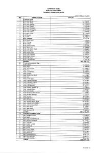


![[Read] PDF International Marketing - By Dana-Nicoleta ...](https://p.pdfkul.com/img/300x300/read-pdf-international-marketing-by-dana-nicoleta-_59e04c751723dd690db3f3ce.jpg)


