The Fed’s perceived Phillips curve: Evidence from individual FOMC forecasts
Peter Tillmann1 Justus Liebig University Giessen October 2009
Abstract: This note uncovers the Phillips curve trade-off perceived by U.S. monetary policymakers. For that purpose we use data on individual forecasts for unemployment and inflation submitted by each individual FOMC member, which was recently made available for the period 19921998. The results point to significant changes in the perceived trade-off over time with the Phillips curve flattening and the implied NAIRU falling towards the second half of the sample. Hence, the results suggest that policymakers were aware of these changes in real-time. Keywords: inflation forecast, NAIRU, Phillips curve, monetary policy, Federal Reserve JEL classification: E43, E52
1
I thank Sarah Lein and Martin Mandler for very helpful comments and suggestions. Contact: Department of Economics, Justus Liebig University Giessen, Licher Str. 62, D-35394 Giessen, Email:
[email protected]
1
Introduction
For central bankers, understanding the short-run trade-off between real economy activity and inflation, also known as the Phillips curve trade-off, is of paramount importance. It is now well known that the Phillips curve flattened since the beginning of the 1980s, a stylized fact first noted by Atkeson and Ohanian (2001). The period of sustained growth in the second half of the 1990s in the absence of inflationary pressure is widely believed to reflect a further significant structural change in the underlying trade-off. Due to favorable productivity shocks, the argument goes, the Non-Accelerating Rate of Unemployment (NAIRU) fell. When did policymakers notice this change and, if so, how did they react?2 These questions are difficult to address based on aggregate macroeconomic data, let alone ex-post revised data. Researchers typically focus on verbal transcripts to illustrate how uncertainty about the Phillips curve affected Federal Reserve decision making. Meade and Thornton (2008), for example, study the debate within the Federal Open Market Committee (FOMC) about the Phillips curve in the 1990s. They document that the FOMC transcripts contain a dramatic increase in references to keywords such as "potential output", "Phillips curve", and "NAIRU" towards the second half of the 1990s. They also list examples of FOMC members expressing doubt about the reliability of the Phillips curve as a guideline for interest rate policy. An alternative approach is offered by Ball and Tchaidze (2002). They show that a standard Taylor rule can replicate interest rate setting during the late 1990s only once a falling NAIRU is taken into account. In the 1990s, the Federal Reserve Board’s main macroeconometric model, FRB/US, underwent various changes. Tetlow and Ironside (2007) document 30 model vintages. They show that the changing model properties are consistent with a falling NAIRU and a flatter Phillips curve. This paper addresses these potential changes in the unemployment-inflation nexus and elicits the perception of the Phillips curve trade-off implicit in forecasts of inflation and unemployment of each individual member of the FOMC. Instead of relying on aggregate data or verbal statements, this paper infers the real-time beliefs about this issue directly from policymakers’ quantitative forecasts. For this purpose, we employ 2
This uncertainty about the Phillips curve relation let research such as Gorodnichenko and Shapiro (2007) refer to monetary policy as the "growth gamble" of the Fed in the second half of the 1990s. For a survey on the emergence of the New Economy and the response of monetary policy see Wynne (2002).
2
a data set on individual forecasts, that is, forecasts for inflation and unemployment of each individual FOMC member, which was recently made available in Romer (2009). By submitting these forecast twice a year, each FOMC member is forced to reveal his notion of the trade-off between real activity and inflation. The data set covers the period 1992-1998, which is the period of heightened uncertainty about the usefulness of the Phillips curve. We estimate a Phillips curve based on the real-time output gap as a driving variable and, alternatively, with unemployment as the measure of real activity. The former specification allows us to infer changes in the slope over time. The latter specification can be used to elicit the NAIRU implied by each member’s combination of unemployment and inflation forecasts The results point to significant changes in the slope of the perceived Phillips curve over time with the Phillips curve flattening towards the second half of the sample. While individual forecasts reflect a positively sloped Phillips curve in the early 1990s, there appears to be no significant relation between inflation and the output gap towards the end of the sample. The estimates also suggest that the NAIRU fell over time from about 6.9% in 1992-1994 to 5.3% after 1996. Hence, we conclude that the FOMC forecasts are consistent with the notion that the Phillips curve changed during the second half of the 1990s and that, on average, FOMC members took that into account when submitting their forecasts. This note is organized as follows. Section two introduces FOMC forecasts and presents the data set. Section three contains the empirical approach and discusses the results. Section four draws some tentative conclusions.
2
FOMC forecasts
Twice a year at its February and July meetings the FOMC publishes the monetary policy report to congress (Humphrey-Hawkins report). It contains forecasts of, among other variables, unemployment and the inflation rate. Each FOMC member submits her own forecasts, after intensive briefing by the FOMC staff. The staff publishes its own set of forecasts in the Greenbook, which is continuously available to FOMC members. Until recently, however, individual forecasts were kept secret. The published report only contains a range of forecasts and the midpoint of this range, also known as the central tendency.
3
These data received some attention in recent years. Gavin (2003) evaluates the information content of the central tendency and the FOMC’s forecasting record, while Gavin and Mandal (2003) compare forecast accuracy between the FOMC, the private sector, and the staff. Likewise, Romer and Romer (2008) compare FOMC forecasts with Federal Reserve staff forecasts. They provokingly argue that the FOMC forecasts do not contain useful information beyond that already incorporated in staff forecasts. Differences between FOMC and staff forecasts are shown to predict monetary shocks. Gavin and Pande (2008) use data from the survey of professional forecasters to mimic the FOMC’s forecasting method and analyse the different measures of forecast consensus. Recently, Romer (2009) constructs a data set containing each individual FOMC forecast for the period 1992-1998. With this publication, the interest in FOMC forecasting is most likely to be revived. The present paper is the first attempt to use this data set.3 We use this data set to uncover policymakers’ beliefs about the Phillips curve trade-off. By setting a forecast of unemployment and inflation, each FOMC member implicitly reveals her perception of the short-run trade-off between these two variables.4 In this respect, the short sample period available to the researcher is not a serious restriction as this time span reflects the period of policymakers’ heightened uncertainty about possible changes in the trade-off due to favorable shift in productivity. In the July report, the FOMC prepares forecasts for the following calender year (this forecast will be indexed by | + 18 hereafter) and the current calender year (indexed by | + 6). The February report contains forecasts for the current calender year ( |+12). The inflation forecast is the expected forth-quarter-to-fourth-quarter change of the CPI, while the unemployment forecast refers to the rate of unemployment in the last quarter of the year. The forecasts are supposed to be conditional on each member’s own judgement of the "appropriate policy" path over the forecast horizon. For each of the three different forecasts per year, i.e. one at the February meeting and two at the July meeting, the data set contains 120 pairs of forecasts for inflation and the unemployment rate. We use these individual FOMC forecasts to address the following questions. First, how do FOMC members perceive the trade-off between the 3
All data series about FOMC forecasts used in this paper are available at David Romer’s website under http://elsa.berkeley.edu/~dromer/. 4 The data set does not contain forecasts from the chairman.
4
output gap and inflation? Put differently, is there a systematic relationship between their inflation forecast and the last observation on the output gap prior to submitting the inflation forecast? Second, how does the perceived slope of the Phillips curve change over time? Third, what is the NAIRU implied by the combined forecasts for inflation and unemployment. Note that this paper does not evaluate issues of forecast accuracy or forecast rationality. Throughout the exercise we maintain the assumption that strategic motives in forecasting were absent.
3
Empirical evidence
We proceed in two steps. In the first step, the inflation forecasts are related to past inflation and the output gap in order to infer the slope of the Phillips curve that is consistent with each member’s forecast. In a second step, the inflation forecast is related to the unemployment forecast. This allows us to extract the NAIRU implied by each individual set of forecasts.
3.1
The Phillips curve as implied by FOMC forecasts
The reduced form specification used in this section relates the February or, alternatively, the July inflation forecast, |+12 or |+6 , to the last observations on inflation and the output gap available at each FOMC meeting. For the February forecast, the model is |+12 − |−12 = 0 + 1 |−3 +
(1)
while the specification for the July forecast is given by |+6 − |−12 = 0 + 1 |−3 +
(2)
A similar specification is used frequently in the literature, e.g. Clark and McCracken (2006). The last year-on-year inflation figure available to the policymaker at the time of the meeting is denoted by |−12 and |−12 . The output gap over the proceeding quarter is |−3 or |−3 . We also include a constant 0 . Data on inflation is taken from the FRED database at the Federal Reserve Bank of St. Louis. The output gap, i.e. the percentage deviation of output from potential, is taken from the Fed’s Greenbook. Hence, is corresponds to the real-time data the FOMC members had at hand when formulating forecasts. This data comes from the real-time 5
database at the Federal Reserve Bank of Philadelphia. If FOMC members raise their inflation forecast in light of current output gap data, the coefficient 1 is expected to be positive. To the extent the decision makers loose faith in the Phillips curve relationship, the coefficient 1 will fall over time. The results are presented in table (1). In almost all specifications, the slope coefficient is significantly positive. Moreover, the Phillips curve flattens over time. Take the February forecasts as an example. In the early years of the sample, i.e. 1992-1994, the slope is 1 = 021. This coefficient falls to 014 in the 1995-1998 subsample. Note that this turns out to be a significantly lower slope coefficient. When forecasts from the February and the July meetings are included jointly, the drop in the implied slope coefficient becomes even more pronounced. It falls from 013 in 1992-1994 to 005 in 1995-1998. This is a key result of the paper. The Phillips curve that is consistent with each member’s submitted inflation forecasts flattens in the second half of the 1990s. Not surprisingly, the share of variation explained by this simple model is rather low. The 2 falls to even lower levels in the later years of the sample. This also indicates that the relationship that explains the link between the output gap and the inflation forecast in the early years is no longer able account for the variation of inflation forecasts. Do Federal Reserve governors and regional Federal Reserve Bank presidents disagree about the Phillips curve? Table (2) reports results for each group of FOMC members separately. Interestingly, both groups exhibit coefficients very similar to the overall results from table (1). The fall in the Phillips curve slope appears to be slightly more pronounced for Fed governors than for presidents, but this difference is not statistically significant.
3.2
The NAIRU as implied by FOMC forecasts
The aim of this section is to uncover the perception of the NAIRU implied by each member’s forecast of inflation and the unemployment rate. For that purpose, we again estimate a simple accelerationist Phillips curve regression. In contrast to the previous section, however, we include the unemployment forecast as the real driving variable. The forecast made at each July meeting for the calender year following the meeting, |+18 , is regressed on the July forecast for the current calender year, |+6 , and
6
the forecast for unemployment, also for the current calender year, |+6 |+18 − |+6 = 0 + 1 |+6 +
(3)
Note that all three forecasts entering this equation are formulated at the same FOMC meeting. Based on the parameter estimates we can derive a rough implied estimate of the NAIRU , which is determined by |+18 − |+6 = 0 or = −
ˆ0 ˆ1
(4)
As an alternative specification, we also estimate this regression with the unemployment forecast for the following calender year, i.e. |+18 |+18 − |+6 = 0 + 1 |+18 +
(5)
We are interested in how evolves over time. It is well known that the equilibrium rate of unemployment fell over the second half of the 1990s, see Staiger, Stock, and Watson (2001). It is not clear, however, whether and when FOMC members, probably apart from chairman Greenspan, perceived this fall of the NAIRU in real-time. A first impression can be obtained from a scatter plot of the unemployment forecast against the change in the inflation forecast, see figure (1). Apparently, the relationship became steeper towards the second half of the sample. The baseline regression results are reported in table (3). For the full sample period, the estimated slope coefficient is significantly negative with 1 = −018. Over time the Phillips curve based on the unemployment forecast becomes steeper. The slope increases to −048 in the 1995-1998 subsample. Atkeson and Ohanian (2001) provide evidence of a flatter unemployment-based Phillips curve since the 1980s. Note that the time span we have available here is substantially shorter than in Atkeson and Ohanian (2001). At first sight, however, the steeper Phillips curve disguises the change in the underlying NAIRU, which is in this case more telling than the slope estimates. The implied falls from 693 in the early years to 542 in the later part of the sample. In 1996-1998 subsample the NAIRU falls further to 531. A simple Wald test confirms that this is a significantly lower . This range is consistent with the results based on aggregate data obtained in the literature, see Staiger, Stock, and Watson (2001). Hence, the results reveal that policymakers implicitly base their forecasts of unemployment and inflation on a significantly lower NAIRU in the later part of the 1990s. Again, we 7
can also distinguish between groups of FOMC members. Interestingly, we find a significant drop in the implied NAIRU also for Fed governors, but not for regional Federal Reserve presidents. The results from the alternative specification (5), which features |+18 instead of |+18 , are shown in table (4) and suggest very similar conclusions.
4
Conclusions
This paper investigates how monetary policymakers think about the short-run tradeoff between real activity and inflation, i.e. the Phillips curve. For this purpose, forecasts for unemployment and inflation from each individual FOMC member over the period 1992-1998 are used, which became available recently. When submitting their forecasts, FOMC members appear to have implicitly revealed a significant trade-off. The slope of the Phillips curve, however, is shown to change over time. Inflation forecasts respond less to incoming output gap figures towards the second half of the sample. Alternatively, the joint forecast for inflation and unemployment is consistent with the perception of a falling NAIRU in the post-1995 subsample. The results, therefore, suggest that FOMC members took these changes in the short-run trade-off into account. In their assessment of the Greenspan era, Blinder and Reis (2005, p. 51) discuss the FOMC’s information about the changing trend in productivity and ask "What did Greenspan see that others failed to see?". Here we show that at least the other board members shared his view. The regional Federal Reserve Bank presidents, however, did not. The present paper is a first step to exploit individual FOMC forecasts in order to extract policymakers’ beliefs about unemployment and inflation. Recent papers by Capistrán (2008) and Ellison and Sargent (2009) use the central tendency of FOMC forecasts to identify the degree auf caution and the preference for robustness of FOMC members. The data set collected by Romer (2009) facilitates additional investigations along these lines.
8
References [1] Atkeson, A. and L. E. Ohanian (2001): "Are Phillips Curves Useful for Forecasting Inflation?", Federal Reserve Bank of Minneapolis Quarterly Review 25, 2-11. [2] Ball, L. and R. T. Tchaidze (2002): "The Fed and the New Economy", American Economic Review: Papers & Proceedings 92, 108-114. [3] Blinder, A. S. and R. Reis (2005): "Understanding the Greenspan Standard", in The Greenspan Era: Lessons for the Future, Proceedings of the Jackson Hole Symposium, Federal Reserve Bank of Kansas City, 11-96. [4] Capistrán, C. (2008): "Bias in Federal Reserve Inflation Forecasts: Is the Federal Reserve Irrational or Just Cautious?", Journal of Monetary Economics 55, 14151427. [5] Clark. T. E. and M. McCracken (2006): "The Predictive Content of the Output Gap for Inflation: Resolving In-Sample and Out-of-Sample Evidence," Journal of Money, Credit, and Banking 38, 1127-1148. [6] Ellison, M. and T. J. Sargent (2009): "A defence of the FOMC", unpublished, Oxford University. [7] Gavin, W. T. (2003): "FOMC Forecasts: Is all the Information in the Central Tendency?", Federal Reserve Bank of St. Louis Review, May/June 2003, 27-46. [8] Gavin, W. T. and R. J. Mandal (2003): "Evaluating FOMC forecasts", International Journal of Forecasting (19), 655-667. [9] Gavin, W. T. and G. Pande (2008): "FOMC Consensus Forecasts", Federal Reserve Bank of St. Louis Review, May/June 2008, 149-163. [10] Gorodnichenko, Y. and M. D. Shapiro (2007): "Monetary policy when potential output is uncertain: Understanding the growth gamble of the 1990s", Journal of Monetary Economics 54, 1132-1162. [11] Meade, E. E. and D. L. Thornton (2008): "The Phillips Curve and US Monetary Policy: What the FOMC Transcripts tell us", Paper prepared for the Annual Meeting of the Southern Economic Association. 9
[12] Romer, D. H. (2009): "A New Data Set on Monetary Policy: The Economic Forecasts of Individual Members of the FOMC", NBER Working Paper No. 15208. [13] Romer, C. D. and D. H. Romer (2008): "The FOMC versus the Staff: Where Can Monetary Policymakers Add Value?", American Economic Review: Papers & Proceedings 98, 230-235. [14] Staiger, D., J. H. Stock, and M. W. Watson (2001): "Prices, Wages, and the U.S. NAIRU in the 1990s", in A. B. Krueger and R. Solow (eds.), The roaring nineties: Can full employment be sustained, New York: Rusell Sage Foundation. [15] Tetlow, R. J. and B. Ironside (2007): "Real-Time Model Uncertainty in the United States: The Fed, 1996-2003", Journal of Money, Credit, and Banking 39, 1533-1561. [16] Wynne, M. A. (2002): "How did the emergence of the New Economy affect the conduct of monetary policy in the US in the 1990s?", unpublished, Federal Reserve Bank of Dallas.
10
Table 1: The Phillips curve over different sample periods meeting|horizon
sample
July|+6
1992 - 1998 1992 - 1994 1995 - 1998
Feb|+12
1992 - 1998 1992 - 1994 1995 - 1998
all
1992 - 1998 1992- 1994 1995 - 1998
2
# obs
000
0.00
120
042
0.21
53
0.02
67
003
0.02
120
021
0.16
53
0.11
67
002
0.02
240
013
0.15
105
0.02
135
parameter estimates 0 1 023
(002)∗∗∗
007
(001)
(002)∗∗∗
(005)∗∗∗
025
−004
(004)∗∗∗
017
(004)∗∗∗
082
(022)∗∗∗
002
(005)
020
(002)∗∗∗
058
(010)∗∗∗
013
(003)∗∗∗
Wald
-
(003)
(002)∗ (006)∗∗∗
014
(005)∗∗∗
0.05
(001)∗∗ (003)∗∗∗
005
(003)∗
0.03
Notes: Results from least-squares estimation. Standard errors in parenthesis. A significance level of 1%, 5%, and 10% is indicated by ∗∗∗ , ∗∗ , and ∗ . The hypothesis of the Wald is 1 = 11992−1994 . The column reports the -value.
11
Table 2: The Phillips curve for different groups of FOMC members meeting|horizon
group
sample
all
Governors
1992 - 1998 1992 - 1994 1995 - 1998
all
Presidents
1992 - 1998 1992 - 1994 1995 - 1998
2
# obs
002
0.04
72
010
0.12
33
0.04
39
002
0.01
168
014
0.16
72
0.02
96
parameter estimates 0 1 014
(004)∗∗∗
040
(0161)∗∗∗
009
(005)
022
(023)∗∗∗
065
(012)∗∗∗
015
(004)∗∗∗
Wald
(001)∗ (005)∗∗
005
(005)
0.05
(001) (004)∗∗∗
005
(004)∗∗∗
0.04
Notes: Results from least-squares estimation. Standard errors in parenthesis. A significance level of 1%, 5%, and 10% is indicated by ∗∗∗ , ∗∗ , and ∗ . The hypothesis of the Wald is 1 = 11992−1994 . The column reports the -value.
12
Table 3: The NAIRU for different sample periods and different groups of FOMC members group sample parameter estimates implied Wald 2 # obs 0 1 all
1992 - 1998 1992 - 1994 1995 - 1998 1996 - 1998
Governors
1992 - 1998 1992 - 1994 1995 - 1998 1996 - 1998
Presidents
1992 - 1998 1992 - 1994 1995 - 1998 1996 - 1998
114
(026)∗∗∗
208
(062)∗∗∗
260
(033)∗∗∗
324
(048)∗∗∗
126
(028)∗∗∗
161
(068)∗∗∗
259
(049)∗∗∗
374
(053)∗∗∗
108
(027)∗∗∗
226
(086)∗∗
262
(042)∗∗∗
304
(064)∗∗∗
−018
633
0.19
120
−030
693
0.18
53
−048
542
009
0.47
67
−061
531
009
0.46
50
−021
6.00
0.37
36
−025
6.44
0.28
17
−047
5.51
012
0.60
19
−071
5.27
008
0.79
14
−017
6.35
0.14
84
−032
7.06
0.16
36
−048
5.46
0.11
0.43
48
−057
5.33
0.14
0.36
36
(003)∗∗∗ (009)∗∗∗ (006)∗∗∗ (010)∗∗∗
(005)∗∗∗ (010)∗∗ (009)∗∗∗ (010)∗∗∗
(004)∗∗∗ (013)∗∗ (008)∗∗∗ (013)∗∗∗
Notes: Results from least-squares estimation. Standard errors in parenthesis. A significance level of 1%, 5%, and 10% is indicated by ∗∗∗ , ∗∗ , and ∗ . The hypothesis of the Wald is = 1992−1994 . The column reports the -value.
13
Table 4: The NAIRU for different sample periods and different groups of FOMC members group sample parameter estimates implied Wald 2 # obs 0 1 all
1992 - 1998 1992 - 1994 1995 - 1998 1996 - 1998
Governors
1992 - 1998 1992 - 1994 1995 - 1998 1996 - 1998
Presidents
1992 - 1998 1992 - 1994 1995 - 1998 1996 - 1998
143
(024)∗∗∗
256
(082)∗∗∗
265
(035)∗∗∗
304
(048)∗∗∗
172
(033)∗∗∗
229
(082)∗∗∗
267
(051)∗∗∗
348
(057)∗∗∗
130
(032)∗∗∗
263
(116)∗∗
268
(045)∗∗∗
288
(064)∗∗∗
−023
6.22
0.21
120
−039
6.56
0.16
53
−048
5.22
0.09
0.45
67
−056
5.43
0.10
0.42
50
−029
5.93
0.44
36
−036
6.36
0.35
17
−047
5.68
0.12
0.60
19
−064
5.44
0.09
0.74
14
−021
6.19
0.15
84
−039
6.74
0.12
36
−049
5.47
0.11
0.41
48
−053
5.43
0.16
0.34
36
(004)∗∗∗ (013)∗∗∗ (006)∗∗∗ (005)∗∗∗
(005)∗∗∗ (013)∗∗∗ (009)∗∗∗ (011)∗∗∗
(005)∗∗∗ (018)∗∗ (009)∗∗∗ (013)∗∗∗
Notes: Results from least-squares estimation. Standard errors in parenthesis. A significance level of 1%, 5%, and 10% is indicated by ∗∗∗ , ∗∗ , and ∗ . The hypothesis of the Wald is = 1992−1994 . The column reports the -value.
14
1.2
0.8
0.8
change in inflation forecast
change in inflation forecast
1.2
0.4
0.0
-0.4
-0.8
0.4
0.0
-0.4
-0.8
1992-1998
1992-1994
-1.2
-1.2 4.0
4.5
5.0
5.5
6.0
6.5
7.0
7.5
8.0
4.0
4.5
5.5
6.0
6.5
7.0
7.5
8.0
7.5
8.0
unemployment forecast
1.2
1.2
0.8
0.8
change in inflation forecast
change in inflation forecast
unemployment forecast
5.0
0.4
0.0
-0.4
-0.8
0.4
0.0
-0.4
-0.8
1996-1998
1995-1998 -1.2
-1.2 4.0
4.5
5.0
5.5
6.0
6.5
7.0
7.5
8.0
unemployment forecast
4.0
4.5
5.0
5.5
6.0
6.5
7.0
unemployment forecast
Figure 1: The relation between the unemployment forecast (|+6 ) and the change in the inflation forecast ( |+18 − |+6 ) over alternative subsamples
15