The price of variance risk - Online Appendix Ian Dew-Becker*, Stefano Giglioa, Anh Leb, Marius Rodriguezc September 21, 2016
A.1
Data quality
In this paper, we introduce two new data sets on variance swaps. Given that the data sets are new in the literature, we perform here a number of tests to ensure the quality of the data. Data set 2 (which contains monthly quotes from Markit, aggregated from many dealers) is constructed in the same way and by the same company as the CDS data set from the same firm; this CDS data is known to be a high-quality data set, and is the most widely used data set in research on credit default swaps (Mayordomo, Pena, and Schwartz (2014)). In addition, Markit provides data on the number of quotes obtained from individual dealers, a measure of the depth of the market. The average number of quotes (11) is in the same range (8-15) of the typical number of quotes for CDS spreads, indicating that approximately as many large dealers trade trade in variance swaps as they trade in CDS. Next, we note that unlike in the case of CDS, for the case of variance claims we actually observe the prices in many related markets, which we use to validate our variance swap data. Our data quality check follows four main steps. 1. We confirm that in both data sets prices display a large amount of month to month variation, and the autocorrelations of price changes are close to zero for all maturities (non-zero autocorrelations would indicate that prices are stale). 2. We check that the data in Data set 1 and Data set 2 correspond almost perfectly for the dates and the maturities for which they overlap. * a b c
Northwestern University Kellogg School of Management University of Chicago Booth School of Business Pennsylvania State University Smeal College of Business Board of Governors of the Federal Reserve System
A.1
3. We check that our quotes correspond to actual trades we can observe for a period of time (using data from DTCC on actual transactions). 4. We check the correspondence between variance swap, VIX, and VIX futures data, which overlap for a substantial amount of time and maturities.
A.1.1
Check 1: Price changes in the two data sets
A first data quality check is to ensure that the quotes and prices are updated in a timely way and do not contain stale information.1 To begin with, we verify that prices always change month to month, across all data sets, all securities, and all months (with one single exception in one month and for one maturity only out of 16,928 observations, i.e., in 0.006% of the data). This reflects the fact that our quotes are updated both by the dealers providing quotes to Markit (Data set 2), and by the hedge fund that kept the price records forming Data set 1. A second check is whether prices changes are autocorrelated in any apparent way, in any data set and for any maturity (we have 6 maturities available in the raw data for the first data set, and 10 for the second one). Among the 16 cases, none of the autocorrelations are greater than 0.14, nor statistically significant even at the 10% level. Delayed or incomplete adjustment of reported prices may result in significant measured autocorrelation of price changes, but we find no evidence of this in our data.
A.1.2
Check 2: Data set 1 vs. Data set 2
Next, we check the two data sets against each other. Data set 1 contains monthly data since 1996, whereas Data set 2 contains monthly data since 2006. For the period 2006-2013, the two data sets overlap. The average correlation of prices in the two data sets is 0.999, with the minimum correlation for any maturity occurring for the 30-day maturity, where it drops to 0.997. Price changes are also extremely highly correlated, mostly above 0.99 (with the minimum being 0.98). We also check whether either of the two data sets predicts price changes in the other, a sign of differing quality among the data sets. No price change in one data set significantly or economically predicts price changes in the other data set. 1
For this analysis, we focus only on quotes we actually observe from the source, with no interpolation. Interpolation is however needed for Markit data after 2008, where we observe fixed calendar date maturities. For the Markit dataset, we therefore focus on the maturities around which we see most quotes, so that the interpolation needed is minimal: 1,2,3, 6, 12, 24, 36, 60, 84, 120.
A.2
We conclude that the two data sets essentially agree on all prices reported.
A.1.3
Check 3: Quotes vs. actual trades
As a third quality check, we compare the quotes from our main data set to the prices of actual transactions reported by the Depository Trust & Clearing Corporation (DTCC), which has collected data on all trades of variance swaps in the US since 2013.2 Appendix Figure A.1 shows the distribution of the percentage difference between our quotes and the transaction prices for different maturity baskets. Quotes and transaction prices are in most cases very close, with the median absolute percentage difference across all maturities approximately 1 percent. We conclude that our quotes reflect the prices at which transactions occur with a high degree of accuracy.
A.1.4
Check 4: Variance Swaps vs. VIX vs. VIX Futures
As discussed in the paper, in addition to the two data sets on variance swaps we also observe a term structure of synthetic variance swap prices (VIX) up to 12 months maturity, and of VIX futures (which are exchange-traded contracts) up to 6 months maturity. The three data sets come from entirely independent sources: variance swaps are traded over the counter, the VIX is constructed using options, and VIX futures are exchange traded. These additional data sources are affected by different liquidity and trading setups relative to variance swaps, and if those were particularly important in this market one would expect to find large deviations between these markets and the variance swap market. Instead, we show now that the three markets move essentially together at all maturities. A.1.4.1
Variance Swaps vs. the VIX
The correlation of variance swap prices with the VIX at corresponding maturities is above 0.99 at all maturities. The correlation of price changes is more noisy, but still 0.96 on average across maturities and never below 0.94. None of the price changes in one data set helps in predicting price changes in another data set, indicating that no data set is reacting to information later than the other. We have also compared our variance swap prices with the VIX computed by CBOE (available from 2008 on, and for maturities 3 and 6 months). The CBOE series are denoted VXV and VXMT. The correlation between the 3-month variance swap price and VXV is 2
DTCC was the only swap data repository registered under the Dodd–Frank act to collect data on variance swaps in 2013. The Dodd–Frank act requires that all swaps be reported to a registered data repository.
A.3
.99, and the correlation of changes is .9. The correlation between the 6-month variance swap price and VXMT is .99, and the correlation of changes is .92. A.1.4.2
Variance Swaps vs. VIX futures
Since VIX futures are claims to the VIX in n periods, they are equivalent to forward variance claims with maturity n + 1 (apart of a small convexity adjustment due to the fact that the payoff of VIX futures is expressed in volatility, not variance, units). The correlation of prices is on average 0.993, and always at least 0.992. The correlation of price changes is 0.98 on average, and always at least 0.94. No significant predictive relation exists between price changes from the two sources, except that variance swaps predict VIX futures price changes with a t-stat of 2.08 in only one case (one significant case out of the many predictive tests we ran is not an indication that indeed our variance swap prices data is better than the VIX futures data, as it is likely only due to noise). All of our tests of data quality suggest that the variance swap data is high quality, and displays no indication of bad reporting, stale prices, or differential price behavior due to different liquidity, compared to the other data sources.
A.2
Synthetic variance swap prices
2 using the We construct option-based synthetic variance claims for maturity n, V IXn,t methods described by the CBOE (2009) in their construction of the VIX index, using data from Optionmetrics covering the period 1996 to 2013. 2 for maturity n on date t as In particular, we construct V IXn,t
2 V IXn,t ≡
2 X ∆Ki exp (−nRn,t ) P (Ki ) n i Ki2
(A.1)
i−1 where i indexes options; Ki is the strike price of option i; ∆Ki = Ki+1 −K unless i is the 2 first or last option used, in which case ∆Ki is just the difference in strikes between Ki and its neighbor; Rn,t is the n-day forward yield (from Fama and Bliss (1987)); and P (Ki ) is the midpoint of the bid-ask spread for the out-of-the-money option with strike Ki . The summation uses all options available with a maturity of n days. We deviate slightly here from the CBOE, which drops certain options with strikes very far from the current spot. For each t and n, we require the presence of at least 4 out-of-the-money calls and puts. We create 2 V IXn,t for all monthly maturities by interpolating between available option maturities, using
A.4
the same techniques as the CBOE. Under the assumption that the price of the underlying follows a diffusion (i.e. does not jump), it is the case that V
2 IXn,t
= ≈
EtQ EtQ
�ˆ
t+n
" tn X
σj2 dj
� (A.2)
# RVt+j
(A.3)
j=1
where σt2 is the instantaneous volatility at time t.3 The second line simply notes that the integrated volatility is approximately equal to the sum of squared daily returns (where the quality of the approximation improves as the sampling interval becomes shorter). In other 2 words, when the underlying follows a diffusion, V IXn,t corresponds to the price of an idealized variance swap where the squared returns are calculated at arbitrarily high frequency. 2 prices at the monthly intervals, we also construct forward variance claims, Given V IXn,t V IXFn,t as 2 2 V IXFn,t = V IXn,t − V IXn−1,t (A.4) The forward prices obtained from options are very close to those obtained from variance swaps. Figure 6 in the text compares the two curves for the S&P 500. Figure A.5 compares the curves for the STOXX 50, FTSE 100 and DAX, and shows that the curves are similar for international markets as well (though in that case there is more noise).
A.3
Decomposing the sources of variation of variance swap prices
In this section we investigate whether the variation in variance swap prices is primarily driven by changes in expected future volatility or changes in risk premia.4 Using the definition of forward variance claims, the following identity holds, for each maturity n: " # n−1 X n−j Ftn − Ft0 = [Et RVt+n − RVt ] + −Et rt+1+j (A.5) j=0
where rtn is the one-period return of the n-period forward claim. An increase in the n3
See Carr and Wu (2009). A similar exercise was conducted by Mixon (2007), using S&P 500 options to predict future implied volatility. 4
A.5
period forward variance price must predict either an increase in future realized variance or lower future variance risk premia. Following Fama and Bliss (1987) and Campbell and Shiller (1991), we can then decompose the total variance of Ftn −Ft0 into the component that predicts future RV , and the component that captures movements in risk premia. Note that just as in Fama and Bliss (1987) and Campbell and Shiller (1991), we perform this decomposition in changes (predicting the change in volatility rather than the level of volatility), because the previous empirical literature and our term-structure estimates of Section A.6 highlight the presence of a very persistent factor in the volatility process. The right side of Table A.2 shows this decomposition for different maturities between 1 month and 1 year. We see that most of the variation in variance swap prices can be attributed to movements in the expectation of future realized variance, not risk premia. In particular, at horizons of 3 to 12 months, essentially all the variation in prices is due to variation in expected volatility rather than variation in risk premia. At the same time, we know from Table2 and Figure 1 that prices of both short-term and long-term claims vary substantially: this indicates that the expectation of future realized variance changes dramatically over time. For example, the standard deviation of innovations in the 12-month forward claim is 17 percent per year. Given the finding in this section that the variance of Ft12 is driven entirely by changes in volatility expectations, we see that investors’ expectations of future volatility in fact vary substantially over time.
A.4
More realistic trading strategies
In this section we report the Sharpe ratios on trading strategies designed to capture the pricing of variance risk at different horizons while trying to incorporate more realistic liquidity and trading costs. We consider a trading strategy that rolls over the 1-month variance swap (thus getting exposure to RV), and a trading strategy exposed to news about volatility 6 to 12 months in the future (i.e. a forward on the realized volatility 6 to 12 months ahead). As discussed more below, this 6/12 strategy allows to easily capture the pricing of future volatility while at the same time minimizing the actual amount of trading required (since we consider a 6-month holding period return). We design the trading strategies to have the following features. First, computing their returns does not require interpolation, since they only trade variance swaps at maturities for which we directly observe quotes in our data set. Second, we explicitly account for the bid-ask spread in computing the returns to the strategies. Third, we express our trading strategies directly in terms of variance swaps, not forwards, since what market participants
A.6
can actually trade on the markets are variance swaps. Fourth, we consider 6-month holding period returns for the 6/12 strategy, so that all trades involve variance swaps with maturities of either 6 months or 12 months, which are commonly-traded maturities in the variance swap market; in addition, to implement this trading strategy one needs to trade only twice a year, mitigating liquidity concerns. The first trading strategy buys every month a 1-month claim to volatility, collects the payoff at the end of the month (RV), and keeps rolling this investment over. This trading strategy is subject to transaction costs at the time of buying the 1-month variance swap, but incurs no trading cost when collecting realized variance at the end of each month. The 6/12 trading strategy constructs an artificial forward to the variance 6 to 12 months ahead. To do so, it goes long a 12-month variance swap and short a 6-month variance swap. It then holds this position for 6 months. Note that during these 6 months, the RV paid by the two contracts completely offset each other. After 6 months, the 6-month variance swap has expired, and the 12-month swap has become a 6-month variance swap, which is then sold on the market. This strategy therefore incurs transaction costs two times: at inception (for the long 12-month position and the short 6-month position) and at the end of the holding period (when the 6-month variance swap is sold). Table A.1 reports the Sharpe ratios for the two trading strategies. We report the results for both a long and a short position, and also show in the last column the difference in Sharpe ratios. The results show that after accounting for transaction costs, strategies directly exposed to realized variance yield much higher risk premia than strategies exposed to news about future variance (in this case, 6 to 12 months ahead). Accounting for the bid-ask spread has minimal effects on the results, mainly because the bid-ask spread does not vary by maturity within the first year of maturity.
A.5
A no-arbitrage model
In this section, we extend the pricing results from the main text by considering a more formal estimation. We analyze a standard no-arbitrage term structure model for variance swaps. The model delivers implications strongly supportive of our reduced-form results. Because the no-arbitrage model uses the prices of the variance swaps, rather than just their returns, and because it uses a full no-arbitrage structure, it is able to obtain much more precise estimates of risk prices. We show that not only are the risk prices on the level and slope factors statistically insignificant, but they are also economically small. The no-arbitrage model has three additional advantages over the reduced-form analysis:
A.7
it explicitly allows for time-variation in the volatility of shocks to the economy and risk prices, the standard errors for the risk prices take into account uncertainty about the dynamics of the economy (through the VAR), and it links us more directly to the previous literature. Furthermore, because the inputs to the estimation of the no-arbitrage model are the observed variance swap prices rather than monthly returns, the results in this section do not rely on any interpolation and we can simultaneously use the full time series from 1996 to 2013 and every maturity from one month to 14 years. Further results on the details of this model are in section A.6.
A.5.1
Risk-neutral dynamics
We assume that the term structure of variance swaps is governed by a bivariate state vector (s2t , lt2 )0 . Rather than state the factors as a level and slope, we now treat them as a short- and a long-term component, which will aid in the estimation process. s2t is the one-month variance swap price: s2t = EtQ [RVt+1 ]. The other state variable, lt2 , governs the central tendency of s2t . We begin by specifying the conditional risk-neutral mean of the states, 2 Q 0 0 st ρs 1 − ρQ s2t+1 s 2 EtQ lt+1 ρQ 0 lt2 + vlQ = 0 l RVt 0 1 0 0 RVt+1
(A.6)
where vlQ is a constant to be estimated which captures the unconditional mean of realized variance. lt2 can be viewed as the risk-neutral trend of s2t . The first two rows of (A.6) are the discrete-time counterpart to the standard continuous-time setup in the literature, e.g. Egloff, Leippold, and Wu (2010) and Ait-Sahalia, Karaman, and Mancini (2014).5 We diverge from Egloff, Leippold, and Wu (2010) and Ait-Sahalia, Karaman, and Mancini (2014) in explicitly specifying a separate process for realized variance, noting that it is not spanned by the other shocks. The specification of a separate shock to RVt+1 allows us to ask how shocks to both realized variance and the term structure factors are priced.6 Q Q For admissibility, we require that 0 < ρQ s < 1, ρl > 0, and vl > 0. These restrictions ensure that 2 2 risk-neutral forecasts of st and lt , hence variance swap prices at various maturities, are strictly positive. 6 From a continuous-time perspective, it is not completely obvious how to think about a ”shock” to realized variance that is completely transitory. There are two standard interpretations. One is that the innovation in RVt+1 represents the occurrence of jumps in the S&P 500 price. Alternatively, there could be a component of the volatility of the diffusive component of the index that has shocks that last less than one month. At some point, the practical difference between a jump and an extremely short-lived change in diffusive volatility is not obvious. The key feature of the specification is simply that there are shocks to the payout of variance swaps that are orthogonal to both past and future information contained in the term structure. 5
A.8
Given the assumption that s2t = EtQ [RVt+1 ], the price of an n-period variance swap V Stn is
" V Stn = EtQ
n X
#
" n X Q
RVt+i = Et
i=1
# s2t+i−1
(A.7)
i=1
which can be computed by applying (A.6) repeatedly, and which implies that V Stn is affine in s2t and lt2 for any maturity.
A.5.2
Physical dynamics and risk prices
Define Xt ≡ (s2t , lt2 , RVt )0 . We assume that X follows a VAR(1) under the physical measure:7 2 0 ρs 1 − ρQ 0 st s2t+1 s Q 2 2 ρl 0 lt + εt+1 lt+1 = vl + 0 RVt RVt+1 0 ρs,RV 0 0 0 εt+1 ∼ N 0 , Vt (Xt+1 )
(A.8)
(A.9)
0 In our main results, we follow Egloff, Leippold, and Wu (2010) and Ait-Sahalia, Karaman, and Mancini (2014) and assume that the market prices of risk are proportional to the states, so that the log SDF, mt+1 , is mt+1 − Et [mt+1 ] = Λ0t Vt (Xt+1 )−1/2 εt+1 λs st where Λt = λl lt λRV st
(A.10) (A.11)
where the superscript 1/2 indicates a lower triangular Cholesky decomposition. The term Vt (Xt+1 )−1/2 standardizes and orthogonalizes the shocks εt+1 . Λt thus represents the price of exposure to a unit standard deviation shock to each component of Xt+1 . To maintain the affine structure of the model, we need the product Vt (Xt+1 )1/2 Λt to be affine in Xt . The specification for Λt in (A.11) is therefore typically accompanied by a Admissibility requires that vlQ and the feedback matrix in (A.8) be non-negative, which ensures that the forecasts of Xt , and hence future volatility, be strictly positive. 7
A.9
structure for the conditional variance similar to that of Cox, Ingersoll, and Ross (1985),
σs2 s2t 0 σs,RV s2t Vt (Xt+1 ) = 0 σl2 lt2 0 2 2 2 σs,RV st 0 σRV st
(A.12)
which guarantees that Vt (Xt+1 )1/2 Λt is affine in Xt .8
A.5.3
Empirical results
The estimation uses standard likelihood-based methods. Section A.6 describes the details. We use both Data set 1 and Data set 2, meaning that the number of variance swap prices used in the estimation varies over time depending on availability. A.5.3.1
Model fit
Table A.3 reports the means and standard deviations of the variance swap prices observed and fitted by our model together with the corresponding root mean squared errors (RMSE). The average RMSE across maturities up to 24 months is 0.73 annualized volatility points (i.e. the units in Figure 1).9 For maturities longer than 24 months, since we do not have time series of variance swap prices with fixed maturities for the entire sample, we cannot report the sample and fitted moments for any fixed maturity. Instead, we stack all contracts with more than 24 months to maturity into one single series and compute the RMSE from the observed and fitted values of this series. The corresponding RMSE is reported in the last row of Table A.3. At 0.87 percentage points, it compares favorably with the RMSE for the shorter maturities. Table A.3 suggests that our models with two term structure factors plus RV are capable of pricing the cross-section of variance swap prices for an extended range of maturities. Even when maturities as long as 14 years are included in estimation, the data does not seem to call for extra pricing factors. 8
It is important to note that the specifications of Λt in (A.11) and Vt (Xt+1 ) in (A.12) introduce tight restrictions on the difference Et (Xt+1 ) − EtQ (Xt+1 ). In section A.6, we therefore consider two alternative specifications for the variance process Vt (Xt+1 ) and the risk prices Λt that are more flexible in certain dimensions. The results, both in terms of point estimates and standard errors, are essentially identical across the various specifications that we consider, so we report results for this specification here since it is most common in the literature. 9 When we exclude the financial crisis, using a sample similar to that of Egloff, Leippold, and Wu (2010), we obtain an RMSE of 0.33 percentage points, which is nearly identical to their reported value. The increase in fitting error in the full sample is, not surprisingly, brought about by the large volatility spikes that occurred during the crisis.
A.10
A.5.3.2
Risk prices
The steady-state risk prices in the model are reported in Table A.8 along with their standard errors. As in the rest of our analysis, we find clearly that it is the purely transitory shock to realized variance that is priced (RV -risk). In the CIR specification, for example, the Sharpe ratio associated with an investment exposed purely to the transitory RV shock— analogous to the pure RV shock above—is -1.70. In the VAR analysis in the previous section, the pure RV shock had no immediate impact on the level and slope factors, but it could potentially indirectly affect future expected variance through the VAR feedback. In the no-arbitrage model, that effect is shut off through the specification of the dynamics. That is, the RV shock here is completely transitory—it has no impact on expectations of volatility on any future date. The other two shocks are forced to account for all variation in expectations. The fact that the results are consistent between the no-arbitrage model and the reduced-form analysis in the previous section helps underscore the robustness of our findings to different modeling assumptions. In the standard CIR specification, the short- and long-term factors earn risk premia of only -0.11 and -0.18, respectively, neither of which is significantly different from zero. The lack of statistical significance is not due to particularly large standard errors; the standard errors for the risk prices for the s2t and lt2 shocks are in fact substantially smaller than that for the RV shock. Moreover, Sharpe ratios of -0.11 and -0.18 are also economically small. For comparison, the Sharpe ratio of the aggregate stock market in the 1996–2013 period is 0.43. So the risk premia on the short- and long-term components of volatility are between 25 and 42 percent of the magnitude of the Sharpe ratio on the aggregate stock market. On the other hand, the Sharpe ratio for the RV shock is nearly four times larger than that for the aggregate stock market and 10 to 15 times larger than the risk prices on the other two shocks. Our no-arbitrage model thus clearly confirms the results from the previous sections. A.5.3.3
Time-series dynamics
The estimated parameters determining the dynamics of the state variables under the physical measure are (eq. A.8):
2 0 0.82∗∗∗ 0.16∗∗ 0 st s2t+1 2 0 0.98∗∗∗ 0 lt2 + εt+1 lt+1 = 0.99∗∗∗ + RVt+1 0 0.75∗∗∗ 0 0 RVt
A.11
(A.13)
The key parameter to focus on is the persistence of lt2 . For the standard CIR model, the point estimate is 0.9814, with a standard error of 0.0013. At the point estimate, long-term shocks to variance have a half-life of 37 months. That level of persistence is actually higher than the persistence of consumption growth shocks in Bansal and Yaron’s (2004) long-run risk model, and only slightly smaller than the persistence they calibrate for volatility, 0.987. Our empirical model thus allows us to estimate risk prices on exactly the type of long-run shocks that have been considered in calibrations. As we discuss further below, the fact that we find that the long-term shock to volatility is unpriced is strongly at odds with standard calibrations of Epstein–Zin preferences where agents are strongly averse to news about future volatility.
A.6
The no-arbitrage model: estimation details and further results
In this section we report more details of the no-arbitrage model estimation, and consider alternative specifications.
A.6.1
Estimation Strategy
For estimation purposes, a standard and convenient practice of the term structure literature is to assume that some fixed-weights “portfolios” of VS prices are priced perfectly. These portfolios in turn allow one to invert for the latent states which are needed in the computation of the likelihood scores of the data. A challenge in implementing this practice in our context is that for parts of our sample the set of available maturities may change from one observation to the next. In the later part of our sample, we use VS prices with maturities up to 14 years, whereas the longest maturity for the earlier sample is only two years. To tackle this issue, we maintain the assumption from the term structure literature that the current term structure of the VS prices perfectly reveals the current values of states. Nonetheless, we depart from the standard term structure practice by using some time-varying-weights “portfolios” of VS prices in identifying the states at each point in time. The portfolios weights are determined in a way to optimally accommodate different sets of maturities at each point in the sample. To begin, let Dt denote the vector of observed data obtained by stacking up the vector of VS prices on top of the realized variance RVt . Because VS prices are affine in states, we
A.12
can write: Dt = A + BXt .
(A.14)
All entries of the last column of B, except for the last row, are zeros because VS prices are only dependent on s2t and lt2 . In addition, since the last entry of Dt corresponds to RVt , the last row of A is 0 and the last row of B is (0,0,1). Keep in mind that the length of Dt can vary from time to time due to different maturity sets for the observed VS data. We assume that Dt is observed with iid errors: Dto = Dt + et
(A.15)
where Dto denotes the observed counterpart of Dt . Adopting a standard practice in the term structure literature, we assume that the observational errors for the VS prices are uncorrelated and have one common variance σe2 . Because observed RVt is used in practice to determine payoffs to VS contracts, it is natural to assume that RVt is observed without errors. Combined, if a number of J VS prices are observed at time t, the covariance matrix of et , Σe , takes the following form: Σe =
IJ σe2 0J×1 01×J 0
! ,
(A.16)
where IJ denotes the identity matrix of size J. We now explain how we can recursively identify the states. Assume that we already know o conditioning on all information up to time t. Our Xt . Now imagine projecting Xt+1 on Dt+1 assumption (borrowed from the term structure literature) that the current term structure of the VS prices perfectly reveals the current values of the states implies that the fit of this regression is perfect. In other the words, the predicted component of this regression, upon o observing Dt+1 , o o o o )), Et (Xt+1 ) + covt (Xt+1 , Dt+1 )vart (Dt+1 )−1 (Dt+1 − Et (Dt+1
(A.17)
must give us the values for the states at time t + 1: Xt+1 . All the quantities needed to o implement (A.17) are known given Xt . Specifically, Et (Xt+1 ) = K0 +K1 Xt and vart (Dt+1 )= Vt (Xt+1 ) + Σe where Vt (Xt+1 ) is computed according to each of our three specifications for o o the covariance. Et (Dt+1 ) is given by A + BEt (Xt+1 ). And covt (Xt+1 , Dt+1 ) is given by 0 Vt (Xt+1 )B . Clearly, the calculation in (A.17) can be carried out recursively to determine the values of Xt for the entire sample.
A.13
Our approach is very similar to a Kalman filtering procedure apart from the simplifying o o ) ≡ 0. In a term structure fully reveals Xt+1 . That is, Vt (Xt+1 |Dt+1 assumption that Dt+1 context, Joslin, Le, and Singleton (2013) show that this assumption allows for convenient estimation, yet delivers typically highly accurate estimates. o We can view (A.17) as some “portfolios” of the observed data Dt+1 with the weights −1 o o given by: covt (Xt+1 , Dt+1 )vart (Dt+1 ) . As a comparison, whereas the term structure literature typically choose, prior to estimation, a fixed weight matrix corresponding to the lower principal components of the observed data, we do not have to specify ex ante any loading matrix. Our approach determines a loading matrix that optimally extracts information from the observed data and, furthermore, can accommodate data with varying lengths. As a byproduct of the above calculations, we have available the conditional means and o o ). These quantities allow us to compute ) and Vt (Dt+1 variances of the observed data: Et (Dt+1 the log QML likelihood score of the observed data as (ignoring constants): L=
X t
1 1 o o o o − ||vart (Dt+1 )−1/2 (Dt+1 )|. − Et (Dt+1 ))||22 − log|vart (Dt+1 2 2
(A.18)
Estimates of parameters are obtained by maximizing L. Once the estimates are obtained, we convert the above QML problem into a GMM setup and compute robust standard errors using a Newey West matrix of covariance.
A.6.2
Alternative variance specifications
We consider now alternative specifications for Vt (Xt+1 ). Constant variance structure In the first alternative specification, we let Vt (Xt+1 ) be a constant matrix Σ0 . Since both Et (Xt+1 ) and EtQ (Xt+1 ) are linear in Xt , Λt is also linear in Xt . We refer to this as the CV (for constant variance) specification. Flexible structure It is important to note that the specifications of Λt in (A.11) and Vt (Xt+1 ) in (A.12) introduce very tight restrictions on the difference: Et (Xt+1 ) − EtQ (Xt+1 ). Simple algebra shows that the first entry of the product Vt (Xt+1 )1/2 Λt is simply a scaled version of s2t . This means that the dependence of Et (Xt+1 ) and EtQ (Xt+1 ) on lt2 and RVt and a constant must be exactly canceled out across measures. Similar arguments lead to the following restrictions A.14
on the condition mean equation:
s2t+1 2 Et lt+1 = RVt+1 |
0 ρs Q vl + 0 ρs,RV 0 {z } | K0
2 0 1 − ρQ st s 2 ρl 0 lt . RVt 0 0 {z }
(A.19)
K1
So in the CIR specification, the conditional mean equation only requires three extra degrees of freedom in: ρs , ρl , and ρs,RV . The remaining entries to K0 and K1 are tied to their risk-neutral counter parts. By contrast, all entries of K0 and K1 are free parameters in the CV specification. Whereas CV offers more flexibility in matching the time series dynamics of Xt , the parsimony of CIR, if well specified, can potentially lead to stronger identification. However, this parsimony of the CIR specification, if mis-specified, can be restrictive. For example, in the CIR specification, RVt is not allowed to play any role in forecasting X. In the flexible specification, we would like to combine the advantages of the CV specification in matching the time series dynamics of X and the advantages of the CIR specification in modeling time-varying volatilities. For time-varying volatility, we adopt the following parsimonious structure: Vt (Xt+1 ) = Σ1 s2t ,
(A.20)
where Σ1 is a fully flexible positive definite matrix. This choice allows for non-zero covariances among all elements of X. The market prices of risks are given by: Λt = Vt (Xt+1 )−1/2 (Et (Xt+1 ) − EtQ (Xt+1 )),
(A.21)
where the superscript 1/2 indicates a lower triangular Cholesky decomposition. Importantly, we do not require the market prices of risks to be linear, or of any particular form. This is in stark contrast to the CIR specification which requires the market prices of risks to be scaled versions of states. As a result of this relaxation, no restrictions on the conditional means dynamics are necessary. Aside from the non-negativity constraints, the parameters K0 , K1 that govern Et (Xt+1 ) = K0 +K1 Xt are completely free, just as in the CV specification. In particular, RVt is allowed to forecast X and thus can be important in determining risk premiums. We label this specification as the FLEX specification (for its flexible structure).
A.15
A.6.3
Empirical results under alternative specifications
Q Q Table A.4 reports the risk neutral parameters of our no arbitrage models: ρQ s , ρl , and vl . As expected, these parameters are very strongly identified thanks to the rich cross-section of VS prices used in the estimation. Recall that our risk-neutral construction is identical for all three of our model specifications. As a result, estimates of risk neutral parameters are nearly invariant across different model specifications. Q The effect of including the crisis is that the estimates for ρQ s and vl are higher, whereas Q the estimate of ρQ s is the same. A higher vl is necessary to fit a higher average VS curve. A 2 higher estimate for ρQ s implies that risk-neutral investors perceive the short-run factor st as more (risk-neutrally) persistent. In other words, movements of the one-month VS price (s2t ) will affect prices of VS contracts of much longer maturities. We report the time series parameters—K0 , K1 , and other parameters that govern the conditional variance Vt (Xt+1 )—for the CV, CIR, and FLEX specifications in Tables A.5, A.6, and A.7, respectively. It is notable that the point estimates and standard errors are similar across the various specifications for the variance process (and hence the physical dynamics), emphasizing the results of our findings. Finally, the table also shows that the results are similar regardless of whether the financial crisis is included in the estimation sample. Since the financial crisis was a period when the returns on variance swaps were extraordinarily high, excluding it from the data causes to estimate risk prices that are even more negative than in the full sample.
A.7
Calibration and simulation of the models
This section gives the details of the three models analyzed in the main text.
A.7.1
Long-run risk (Drechsler and Yaron)
Our calibration is identical to that of Drechsler and Yaron (DY; 2011), so we refer the reader to the paper for a full description of the model. We have confirmed that our simulation matches the moments reported in DY (tables 6, 7, and 8, in particular).
A.16
In DY there is a vector of state variables, Xt , that follows a VAR(1), Yt = µ + F Yt−1 + Gt zt+1 + Jt+1
(A.22)
zt ∼ N (0, I)
(A.23)
Gt G0t = h + hσ σt2
(A.24)
PNi,t+1 where σt2 is one of the elements of Yt and Jt+1 is a vector with components Ji,t+1 = j=1 ξj,i , where Ni,t+1 is a Poisson-distributed random variable and ξj,i is the size of each jump. The jump intensity follows the process λt = l0 + l1 σt2 . Using the standard linear approximations applied in models such as this one (e.g. Bansal and Yaron (2004)), one may show that the log return on equity takes the form re,t+1 = r¯e + ry Yt + rz (Gt zt+1 + Jt+1 )
(A.25)
where the coefficients r¯e , ry , and rz are solved for as part of the equilibrium. Following DY, we then calculate the realized variance in period t (i.e. RVt from above) as RVt = rz Gt−1 G0t−1 rz0 + rz Jt Jt rz0 � 0 2 = rz h + hσ σt−1 rz + rz Jt Jt rz0
(A.26) (A.27)
The implicit assumption then is that the zt+1 shocks occur diffusively during a period, while the jumps happen on a single day. It is straightforward to calculate the price of such a claim using the formula for the pricing kernel provided in DY (eq. 6; or, alternatively, using the risk-neutral dynamics in eq. 20).
A.7.2
Time-varying disasters with Epstein–Zin (Wachter)
The key equations driving the economy are ∆ct = µ∆c + σ∆c ε∆c,t + J∆c,t Ft = (1 − ρF ) µF + ρF Ft−1 + σF ∆dt = λ∆ct
p Ft−1 εF,t
(A.28) (A.29) (A.30)
where ε∆c,t and εF,t are standard normal innovations. This is a discrete-time version of Wachter’s setup, and it converges to her model as the length of a time period approaches A.17
zero. The model is calibrated at the monthly frequency. Conditional on a disaster occurring, J∆c,t ∼ N (−0.15, 0.12 ) . The number of disasters that occurs in each period is a Poisson variable with intensity Ft . The other parameters are calibrated as: Parameter
Value
Parameter
Value
µ∆c σF ρF
0.0252/12 0.067/12 exp(−0.08/12)
σ∆c λ µF
0.02/sqrt(12) 2.6 0.0355/12
Using the Campbell–Shiller approximation to the return on equity, one may show that the log price/dividend ratio follows pdt = z0 + z1 Ft
(A.31)
In the absence of a disaster, we treat the shocks to consumption and the disaster probabil2 ity as though they come from a diffusion, so that the realized variance is θ2 z02 σF2 Ft−1 + λσ∆c (where θ ' 1 is the linearization parameter from the Campbell–Shiller approximation). When a disaster occurs, we assume that the largest daily decline in the value of the stock market is 10 percent. So, for example, a 30-percent decline would be spread over 3 days. The results are largely unaffected by the particular value assumed. The realized variance 2 − (0.1) J∆c,t (assuming J∆c,t ≤ 0). when a disaster occurs is then θ2 z02 σF2 Ft−1 + λσ∆c The model is solved analytically using methods similar to those in DY. Specifically, household utility, vt , is vt = (1 − β) ct +
β log Et [exp ((1 − α) vt+1 )] 1−α
(A.32)
α is set to 4.9 and β = exp (−0.012/12). The recursion can be solved because the cumulantgenerating function for a poisson mixture of normals (the distribution of J∆c ) is known analytically (again, see DY). The pricing kernel is Mt+1 = β exp (−∆ct+1 )
exp ((1 − α) vt+1 ) Et [exp ((1 − α) vt+1 )]
(A.33)
Asset prices, including those for claims on realized variance in the future, then follow immediately from the solution of the lifetime utility function and cumulant-generating function for J∆c . The full derivation and replication code is available upon request. As with the DY model, we checked that the moments generated by our solution to the model match those reported by Wachter. We confirm that our results are highly similar, A.18
in particular for her tables 2 and 3, though not identical since we use a different disaster distribution.
A.7.3
Disasters with habit formation (Du)
We calibrate the model exactly as in Du (2011). We also use the formulas he provides for the processes driving equity returns and the pricing kernel. As with the other disaster model, we assume that the maximum equity return on a single day is 10 percent. For a grid of possible values of the only state variable, γt , we numerically integrate realized volatility and γ itself under the physical and risk-neutral distributions. This allows us to calculate numerical expected values of realized volatility under the physical and risk-neutral distributions, yielding variance forward prices. The model is simulated at a daily frequency for the numerical calculations.
A.7.4
Disasters with time-varying recovery (Gabaix) ∆ct = µ∆c + ε∆c,t + J∆c,t
(A.34)
¯ + ρL Lt−1 + εL,t Lt = (1 − ρL ) L
(A.35)
∆dt = λε∆c,t − L × 1 {J∆c,t 6= 0}
(A.36)
The model is calibrated at the monthly frequency. Conditional on a disaster occurring, J∆c,t ∼ N (−0.3, 0.152 ) . The probability of a disaster in any period is 0.01/12. The other parameters are calibrated as: Parameter
Value
µ∆c stdev(ε∆c ) ρL ¯ L
0.1/12 √ 0.02/ 12 0.871/12 0.5 0.04 5
stdev(εL ) λ
Agents have power utility with a coefficient of relative risk aversion of 7 and a time discount factor of 0.961/12 .
A.19
References Ait-Sahalia, Yacine, Mustafa Karaman, and Loriano Mancini, “The Term Structure of Variance Swaps, Risk Premia and the Expectations Hypothesis,” 2014. Working paper. Bansal, Ravi and Amir Yaron, “Risks for the Long Run: A Potential Resolution of Asset Pricing Puzzles,” Journal of Finance, 2004, 59 (4), 1481–1509. Campbell, John Y. and Robert J. Shiller, “Yield Spreads and Interest Rate Movements: A Bird’s Eye View,” Review of Economic Studies, 1991, 58(3), 495–514. Carr, Peter and Liuren Wu, “Variance Risk Premiums,” Review of Financial Studies, 2009, 22(3), 1311–1341. Cox, John C., Jr. Jonathan E. Ingersoll, and Stephen A. Ross, “A Theory of the Term Structure of Interest Rates,” Econometrica, 1985, 53(2), 385–407. Drechsler, Itamar and Amir Yaron, “What’s Vol Got to Do with it?,” The Review of Financial Studies, 2011, 24(1), 1–45. Egloff, Daniel, Markus Leippold, and Liuren Wu, “The Term Structure of Variance Swap Rates and Optimal Variance Swap Investments,” Journal of Financial and Quantitative Analysis, 2010, 45(5), 1279–1310. Exchange, Chicago Board Options, “The CBOE Volatility Index - VIX,” Technical Report, Chicago Board Options Exchange 2009. Fama, Eugene F. and Robert R. Bliss, “The Information in Long-Maturity Forward Rates,” The American Economic Review, 1987, 77(4), 680–692. Mayordomo, Sergio, Juan Ignacio Pena, and Eduardo S. Schwartz, “Are All Credit Default Swap Databases Equal?,” European Financial Management, 2014, 20 (4), 677– 713. Mixon, Scott, “The implied volatility term structure of stock index options,” Journal of Empirical Finance, 2007, 14, 333–354.
A.20
Fig. A.1: Quotes vs. transaction prices
Frequency 10 0
0
2
5
Frequency 4 6
15
8
20
Maturity: 2 months
10
Maturity: 1 month
−.2
0
.2 Percentage difference Mean=.7%, Stdev=5.98%
.4
−.1
0 .1 Percentage difference Mean=−.3%, Stdev=3.95%
Maturity: 4−6 months
Frequency 10 0
0
10
5
Frequency 20 30
15
40
50
20
Maturity: 3 months
.2
−.04
−.02
0 .02 Percentage difference Mean=.45%, Stdev=2.38%
.04
.06
0
.2
.8
1
Maturity: 13−24 months
0
0
10
10
Frequency
Frequency 20
20
30
30
Maturity: 7−12 months
.4 .6 Percentage difference Mean=1.33%, Stdev=7.78%
−.1
0
.1 Percentage difference Mean=1.71%, Stdev=4.66%
.2
.3
−.2
0
.6
.8
Maturity: 60+ months
0
0
50
10
Frequency 20
Frequency 100 150
30
200
40
250
Maturity: 25−60 months
.2 .4 Percentage difference Mean=.92%, Stdev=6.4%
0
.2
.4 Percentage difference Mean=1.84%, Stdev=8.99%
.6
.8
−.02
−.01 0 Percentage difference Mean=−.45%, Stdev=.67%
.01
The figure shows the distribution of percentage difference between variance swap price quotes and actual transaction prices, computed as (transaction price - quote)/quote. The quotes are our main sample, while transaction prices are obtained from the DTCC and begin in 2013. Each panel shows the histogram for a different bucket of maturity of the variance swap contracts.
A.21
Fig. A.2: Distribution of maturity of CBOE options, weighted by open interest 9
8
7
Maturity (months)
6
5
4
3
2
1
0 1996 1997 1998 1999 2000 2001 2002 2003 2004 2005 2006 2007 2008 2009 2010 2011 2012 2013 2014 Average
75th percentile
The figure shows at each point in time the average and 75th percentile of the maturity of options traded on the CBOE, weighted by open interest.
Table A.1: Accounting for transaction costs Long position
1mo
Midpoint -1.32 Using bid-ask spread -1.64
12/6mo
Diff.
0.11 -0.09
-1.44 -1.56
Short position
1mo
12/6mo
Diff.
Midpoint Using bid-ask spread
1.32 1.00
-0.11 -0.31
1.44 1.32
The Table reports annualized Sharpe ratios of two different trading strategies described in Appendix A.4. The trading strategy denoted “1mo” rolls over a long 1-month variance swap. The trading strategy denoted “12/6mo” consists in going long a 12-month variance swap and short a 6-month variance swap, holding for 6 months, and liquidating the position. The return therefore corresponds to the 6-month holding period return on a forward claim to realized variance 6 to 12 months ahead. The top panel reports the Sharpe ratio on long positions, the bottom panel on short positions. In each panel, the “midpoint” Sharpe ratio ignores transaction costs, whereas the “bid-ask” Sharpe ratio considers the bid-ask spread in computing the transaction cost of the strategy. The last column of the table reports the difference in Sharpe ratios between the two strategies.
A.22
Fig. A.3: Annualized Sharpe ratios for unscaled returns on forward variance claims Sharpe Ratio (annualized), 1996:01 - 2013:10
0.6 0.4 0.2 0 -0.2 -0.4 -0.6 -0.8 -1 -1.2 -1.4 1
2
3
4
5
6
7
8
9
10
11
12
Maturity (months)
The figure shows the annualized Sharpe ratio for unscaled returns on forward variance claims.
Fig. A.4: Sharpe ratios for VIX forwards using daily data Sharpe Ratio (annualized), 1997:10 - 2013:08
1
0.5
0
-0.5
-1
-1.5
1
2
3
4
5
6
7
8
9
10
11
12
Maturity (months)
The figure shows the annualized Sharpe ratio for VIX claims, calculated using the VIX formula and CBOE option data at monthly maturities. The figure computes monthly returns at the daily frequency. Standard errors are Hansen-Hodrick standard errors with 21 lags (the number of trading days in each month) to take into account the overlap.
A.23
Fig. A.5: International forward variance claim prices from options and variance swaps Period: 2013:4 - 2014:02 25 24 23 22 21 20 19 18 17 16 15
STOXX (options) STOXX (VS)
0
2
4
6
8
10
12
Maturity (months) Period: 2013:4 - 2014:02 21 20 19 18 17 16 15 14 13 12 11
FTSE (options) FTSE (VS)
0
2
4
6
8
10
12
Maturity (months) Period: 2013:4 - 2014:02 24
22
20
18
16
14 DAX (options) DAX (VS)
12
0
2
4
6
8
10
12
Maturity (months)
In each panel (corresponding to STOXX 50, FTSE 100 and DAX), the solid line plots average prices of forward variance claims calculated using the formula for the VIX index and data on international option prices from Optionmetrics. The dotted line plots the average prices of the same claims computed from international variance swaps. The sample covers the period 2013:4-2014:2.
A.24
Fig. A.6: VIX futures vs. forward variance swap prices Period: 2006:10 - 2012:09 55 50 45 40 35 30 25 20 15 10
2-month zero-coupon variance swap 1-month VIX future
2007
2008
2009
2010
2011
2012
Period: 2006:10 - 2012:09 45
40
35
30
25
20
15 7-month zero-coupon variance swap 6-month VIX future
10
2007
2008
2009
2010
2011
2012
the top panel plots the time series of the 2-month forward variance swap and the 1-month VIX future price from the CME, in annualized volatility terms. The bottom panel plots the time series of the 7-month forward variance swap and the 6-month VIX future price from the CME, in annualized volatility terms. The sample covers the period 2006:10-2012:9.
A.25
Table A.2: Predictive regressions
Horizon
Predictor: Slope and Curvature
(months)
Dep var: RVt+n − RVt
1
Predictor: Ftn − Ft0 Dep var: RVt+n − RVt
Dep var: −
coeff.
R2
coeff.
0.08
0.17
0.63∗∗∗
0.07
0.37∗ (0.22)
0.71∗∗∗
0.18
0.04
(0.17) 0.31
0.83∗∗∗
0.24
0.36
0.01
0.001
(0.09) 12
0.38
0.05 (0.09)
1.10∗∗∗
0.41
0.17 (0.14)
0.95∗∗∗
0.34
0.29∗ (0.17)
(0.14) 6
0.001
(0.09)
-0.10 (0.09)
Results of regressions forecasting changes in realized variance. The left side reports the R2 of a regression of changes in realized volatility between month t and month t + n on the level and the slope at time t. The right side reports the coefficients of univariate regressions of changes in realized volatility (left column) and returns to volatility claims from t to t + n (right column) on the difference between the forward prices of maturity n (Ftn ) and realized volatility (Ft0 ) at time t. * indicates significance at the 10-percent level, ** the 5-percent level, and *** the 1-percent level.
Table A.3: Average prices and pricing errors for the no-arbitrage model
Maturity (months) 1 2 3 6 12 24 >24
n−j rt+1+j
R2
0.22
3
j=0
R2
(0.22) 2
Pn−1
Sample Mean 21.24 21.89 22.22 22.75 23.20 23.65
Fitted
Std 8.00 7.55 7.25 6.64 6.06 5.58
Mean 21.70 21.88 22.04 22.42 22.99 23.87
Std 7.86 7.55 7.30 6.74 6.11 5.45
RMSE 1.00 0.33 0.40 0.63 0.53 0.61 0.87
Prices are reported in annualized volatility terms. The RMSE is calculated using the deviation of the fitted price from the sample price in annualized voaltility terms.
A.26
Table A.4: Risk neutral parameters
1996:2007 ρQ s
Specifications
1996:2013
ρQ l 0.99∗∗∗
vlQ 0.65∗∗∗
ρQ s
ρQ l
vlQ
0.14
0.83∗∗∗ 0.07
0.99∗∗∗ 0.01
1.01∗∗ 0.48
0.00
CV
Est. Stderr.
0.66∗∗∗ 0.06
CIR
Est. Stderr.
0.68∗∗∗ 0.05
0.99∗∗∗ 0.00
0.65∗∗∗ 0.14
0.84∗∗∗ 0.06
0.99∗∗∗ 0.01
0.99∗∗ 0.44
FLEX
Est. Stderr.
0.66∗∗∗ 0.06
0.99∗∗∗ 0.00
0.64∗∗∗ 0.14
0.83∗∗∗ 0.07
0.99∗∗∗ 0.01
1.01∗∗ 0.47
The table reports the risk-neutral estimated dynamics of the term structure model, for the three specifications CV, CIR and FLEX, and separately for the full sample (1996-2013) and the pre-crisis sample (1996-2007).
Table A.5: Time series parameter estimates for the CV specification
Sample
K0 Est.
1996:2007 Std. err.
Est. 1996:2013 Std. err.
Σ∗
K1
6.49∗∗∗ 3.36∗∗∗ 1.98
0.65∗∗∗ 0.08 0.56∗∗∗
0.14∗∗ 0.83∗∗∗ 0
0.03 0.02 0.12
15.42∗∗∗ 3.87∗∗∗ 10.57∗∗∗
0 5.25∗∗∗ -2.62
0 0 14.08∗∗∗
2.42 1.12 2.11
0.08 0.10 0.07
0.07 0.08 -
0.12 0.07 0.10
3.23 0.73 2.36
0.73 2.63
2.07
8.99∗∗∗ 2.43∗∗∗ 5.67∗
0.56∗∗∗ 0 0.20
0.08 0.91∗∗∗ 0
0.19∗∗ 0.06∗∗∗ 0.57∗∗∗
20.59∗∗∗ 3.26 30.00∗∗
0 7.04∗∗∗ -2.14
0 0 25.49∗∗∗
2.48 0.90 2.92
0.13 0.13
0.05 0.03 -
0.09 0.01 0.15
5.07 2.09 13.38
0.97 2.94
4.23
The table reports the time-series parameter estimates for the CV specification. Σ∗ is the lower triangular Cholesky decomposition of Σ0 . For admissibility, K0 and K1 are constrained to be non-negative. Those entries for which the non-negativity constraint is binding are set to zero and thus standard errors are not provided. The table reports the estimates separately for the full sample (1996-2013) and the pre-crisis sample (1996-2007).
A.27
Table A.6: Time series parameter estimates for the CIR specification
Sample
K0 Est.
1996:2007 Std. err.
Est. 1996:2013 Std. err.
Σ∗
K1
0 0.65∗∗∗ 0
0.66∗∗∗ 0 0.69∗∗∗
0.32∗∗∗ 0.99∗∗∗ 0
0 0 0
5.16∗∗∗ 0 3.53∗∗∗
0 0.98∗∗∗ 0
3.53∗∗∗ 0 6.74∗∗∗
0.14 -
0.07 0.01
0.05 0.00 -
-
1.82 1.18
0.23 -
1.18 1.69
0 0.99∗∗ 0
0.82∗∗∗ 0 0.75∗∗∗
0.16∗∗ 0.98∗∗∗ 0
0 0 0
7.17∗∗ 0 9.42∗
0 1.42∗∗ 0
9.42∗ 0 23.56∗
0.44 -
0.04 0.09
0.06 0.00 -
-
2.84 5.42
0.58 -
5.42 12.88
The table reports the time-series parameter estimates for the CIR specification. The diagonal elements 2 of Σ∗ correspond to the variance parameters σs2 , σl2 , and σRV . The (3,1) entry of Σ∗ correspond to the covariance parameter σs,RV . The table reports the estimates separately for the full sample (1996-2013) and the pre-crisis sample (1996-2007).
A.28
Table A.7: Time series parameter estimates for the FLEX specification
Sample
K0 Est.
1996:2007 Std. err.
Est. 1996:2013 Std. err.
Σ∗
K1
2.31 2.18∗∗∗ 0.11
0.74∗∗∗ 0.09∗ 0.60∗∗∗
0.19∗∗ 0.87∗∗∗ 0
0.01 0 0.13
2.26∗∗∗ 0.58∗∗∗ 1.56∗∗∗
0 0.78∗∗∗ -0.24
0 0 2.04∗∗∗
1.49 0.81 0.75
0.08 0.05 0.08
0.08 0.06 -
0.08 0.09
0.42 0.08 0.29
0.08 0.31
0.27
4.54∗∗∗ 1.37∗∗ 0.67∗∗∗
0.68∗∗∗ 0 0.36∗∗∗
0.08∗∗ 0.93∗∗∗ 0
0.19∗∗ 0.07∗∗∗ 0.51∗∗
2.59∗∗∗ 0.44∗ 3.32∗∗∗
0 1.09∗∗∗ -0.34
0 0 3.20∗∗∗
1.30 0.55 0.05
0.08 0.11
0.04 0.02 -
0.08 0.02 0.20
0.48 0.23 1.24
0.12 0.43
0.48
The table reports the time-series parameter estimates for the FLEX specification. Σ∗ is the lower triangular Cholesky decomposition of Σ0 . For admissibility, K0 and K1 are constrained to be non-negative. Those entries for which the non-negativity constraint is binding are set to zero and thus standard errors are not provided. The table reports the estimates separately for the full sample (1996-2013) and the pre-crisis sample (1996-2007).
Table A.8: Annualized steady state risk prices, all specifications
1996:2007
1996:2013
Specifications
Sources of risks
Estimates
Standard Error
Estimates
Standard Error
CV
s2t -risk lt2 -risk RV-risk
-0.23 0.05 −2.78∗∗∗
0.22 0.18 0.65
-0.08 -0.21 −1.44∗∗∗
0.14 0.14 0.43
CIR
s2t -risk lt2 -risk RV-risk
-0.18 0.04 −3.92∗∗∗
0.36 0.14 0.91
-0.11 -0.18 −1.70∗∗∗
0.31 0.12 0.48
FLEX
s2t -risk lt2 -risk RV-risk
-0.23 0.06 −3.17∗∗∗
0.30 0.22 0.78
-0.14 -0.17 −1.69∗∗
0.16 0.19 0.73
Estimates of steady-state risk prices from the no-arbitrage model. Risk prices are annualized by multiplying √ by 12. *** denotes significance at the 1-percent level. Results are reported for the full sample (19962013), and restricted to 1996-2007.
A.29