The Time Value of Housing: Historical Evidence on Discount Rates∗ Philippe Bracke†
Edward W. Pinchbeck‡
James Wyatt§
December 2016 Abstract Most London housing transactions involve trading long leases of varying lengths. We exploit this to estimate the time value of housing—the relationship between the price of a property and the term of ownership—over a hundred years and derive implied discount rates. For our empirical analysis, we compile a unique historical dataset (1987 to 1992) to abstract from the right to extend leases currently enjoyed by tenants. Across a variety of specifications and samples we find that leasehold prices are consistent with a time declining schedule and low long-term discount rates in housing markets.
Keywords housing, leasehold, discount rates JEL codes G10, R30
∗
We thank seminar participants at the LSE/Spatial Economics Research Centre, American Real Estate and Urban Economics Association conference in Reading, Helsinki Government Institute for Economic Research, North American Meetings of the Regional Science Association, as well as Pat Bayer, Dean Buckner, Tom Davidoff, Piet Eichholtz, Hua Kiefer, Colin Lizieri, Sean Holly, Geoff Meen, John Muellbauer, Henry Overman, Olmo Silva, Silvana Tenreyro, and Garry Young for useful comments. Any views expressed are solely those of the authors and cannot be taken to represent those of the Bank of England, its Monetary and Financial Policy Committees or the Prudential Regulation Authority. † Bank of England, email:
[email protected]. Corresponding author. ‡ London School of Economics and Spatial Economics Research Centre, email: e.w.pinchbeck@lse. ac.uk § Parthenia Research and Fellow of the Royal Institution of Chartered Surveyors, email: jwyatt@ parthenia.co.uk
1
Introduction
The shape of discount rate functions — or the term structure of discount rates — provokes considerable research interest across a number of fields. In this paper we use sales of leasehold dwellings to investigate discount rates in housing markets, complementing a recent literature that exploits features of property tenure to estimate market discount rates over long horizons (Wong et al., 2008; Gautier and van Vuuren, 2014; Giglio et al., 2015a; Giglio et al., 2015b; Fesselmeyer et al., 2016). Under a leasehold arrangement a property is owned only for a fixed term so the intuition for why leasehold prices may contain information on discount rates is straightforward. Consider two identical properties, one sold with a fixed term 99-year lease and the other with a 999-year lease.1 Absent any other contractual differences, the gap between the two sale prices must reflect the value of an ownership claim for 900 years, discounted 99 years from now. As with Giglio et al. (2015a) (henceforth GMS), our empirical analysis centres on the English housing market.2 Our contribution can be distinguished by two main differences relative to that paper. First, we compile and refine a unique historical dataset of property sales from 1987-1992 (before the start of the GMS sample), taking advantage of a geographical setting—Prime Central London, the highly urbanised core of London covering Mayfair, Chelsea and Kensington—in which leaseholds account for four-fifths of sales. In England and Wales, reforms in 1993 gave many leaseholders rights to extend their leases or purchase them outright, at a premium agreed with the landlord or decided by a tribunal (if the two parties fail to reach agreement). This option is regarded as valuable, especially for short lease properties, and is exercised for most leases well before the term runs down.3 The historical dataset allows us to abstract from these rights. Second, we concentrate on the shorter end of the term structure and estimate discount rates for leases in the 1-to-99 year range. (With no extension rights before 1993, we find a greater proportion of short leases in the historical data.) This range is likely to be important for public policies that have medium- to long-term consequences — for example infrastructure investments, pension savings, mortgages and related financial products — and given the similarities between very short leases and rentals, our findings also relate to research on rent-price ratios (Smith and Smith, 2006; Gallin, 2008; Campbell et al., 2009; Bracke, 1
Terms of these lengths are commonly granted on new leases in England and Wales. GMS also analyse the housing market in Singapore. 3 A further complication arises in this setting because following the 1993 legislation, a number of real estate companies began to publish and promote graphs purporting to show the relationship between lease length and sales price. These graphs have subsequently become the received wisdom for valuers (and tribunals) in determining the premium for lease extension. Surveyors and agents have used this estimated premium to value and price leasehold properties. 2
1
2015). The principal finding from analysis of our historical sales dataset is that the housing market discount rate schedule over 100 years is declining, with rates net of rental growth around 3% at 100 years. To bridge our paper directly with the GMS study, we next replicate our historical analysis using a sample of sales from the same period (20042013). Crucially, we continue to find a declining term structure of discount rates in this later setting. In terms of discount rate levels, our estimate of 2% at 100 years from this exercise sits comfortably with the GMS finding of 1.9% for the same sample period. By comparing between the two samples (1987-1992 and 2004-2013) we can also shed new light on whether the housing market term structure changes over time. We find that on average housing market discount rates are 1.6 percentage points lower in the later setting, showing for the first time that decisions about the long-run may be context specific. Our regressions use street fixed effects and a large number of property characteristics extracted from sales brochures to disentangle lease length from other neighbourhood and property features. We control for the condition of the property to reflect that a rental externality (Henderson and Ioannides, 1983) may reduce incentives to maintain properties held on short leases. By only comparing leaseholds with other leaseholds we rule out unobserved differences between (and selection into) leasehold and freehold properties, and in restricting attention to hard-to-redevelop flats we control for potential differences in the value of a redevelopment option (Capozza and Sick, 1991). We also take account of residual contractual differences between leases, carefully separating out those sold with a share in the freehold and controlling for rents paid to the freeholder (so-called ground rents) where these are significant. Our setting is one in which very few buyers require mortgage finance so this is also unlikely to be driving results. Additionally, we undertake a number of auxiliary regressions that demonstrate that: (a) conditional on our controls there is no relationship between rental value and lease length for properties in our sample and (b) that our findings are largely insensitive to changes in sample and specifications, including those that (i ) use minimal controls, (ii) use within building variation, (iii) use different time periods or geographies, or (iv) rely on different estimation methods. These results lead us to conclude that omitted variables, for example omitted structural building characteristics or contractual features, are unlikely to be behind our main results. Our results are directly relevant in a number of housing settings, including to individuals in England and Wales who own or are contemplating buying a lease.4 In addition, 4
As we explain elsewhere in the paper, under UK legislation the relationship between lease length and sales price net of the value of the option to extend is a component of the statutory premium to extend a lease. Later in this paper, we show how our findings contrast with conventional practitioner
2
housing market discount rates may be useful in situations that require estimates of real estate values in the far-off future, for example long duration mortgages or housing equity release products (reverse mortgages). In some policy settings outside of housing, such as pension financing, infrastructure investments, and environmental regulation, benefits also accrue only in the far-off future. Debates following the Stern review (Stern et al., 2006; Weitzman, 2007; Nordhaus, 2007) demonstrate that in such cases assumptions about discount rates can be paramount in deciding the optimal policy response. Some authorities, notably the Office of Budgetary Management in the United States, guide policy-makers to use a constant discount rate across all time horizons, while others including in the UK, France, Norway and Denmark have adopted time-declining policy rates (Cropper et al., 2014). Whether our findings can be usefully deployed to these questions depends on the risk characteristics of residential real estate as compared to the ones of the policy application. For instance, infrastructure investments share with real estate some important features such as indivisibility, low liquidity and location specificity; the discount rates patterns uncovered in this paper may therefore provide some additional guidance in cases where housing and infrastructure values are closely related. The paper proceeds as follows. In the next section we describe the institutional setting of the leasehold market in the UK. The following section sets out the data sources that we use for our empirical analysis. We explain our approach in Section 4 before reporting results in Section 5. In Section 6 we discuss threats to identification, paying close attention to findings in the recent literature and outlining techniques and several auxiliary regressions we undertake to resolve them. Section 7 concludes.
2 2.1
Institutional framework Residential leasehold in England and Wales
In England and Wales as many as 1 million houses and 2 million flats are owned under long leases, 40% of recent new build properties are leased, and leaseholds account for around a quarter of residential sales.5 Leaseholds proliferate where populations are most wisdom in this area and lead us to believe that leaseholders commonly overpay for extensions. In a related contribution, Badarinza and Ramadorai (2014) examine some 450 decisions by the UK FirstTier Tribunal—previously known as the Leasehold Valuation Tribunal (LVT)— to settle disputes over the valuation of lease extensions and enfranchisements. Interestingly, these authors contend that the discount rates implicitly adopted by tribunals are high and actually increasing with lease length. 5 Department of Communities and Local Government Table FA1221 (S108): Household type by tenure, 2011-12; housing stock estimates from https://www.gov.uk/government/policies/helping-people-
3
Figure 1: Fraction of leasehold and freehold sales, Land Registry 2013 Notes: The Land Registry contains all residential property sales in England and Wales since 1995. The dataset is available at http://www.landregistry.gov.uk/market-trend-data/public-data. The public version of the dataset only contains an indicator variable which labels properties as freeholds or leaseholds. For the main analysis of this paper, we use proprietary data from real estate agencies in Central London. 1
.8
.6
.4
.2
0
England and Wales
London Freehold
Prime Central London Leasehold
concentrated—they account for around half of the sales in London and over four fifths of sales in Prime Central London (Figure 1). Leasehold ownership is an alternative way to hold residential property outside the more widely studied home-ownership and rental forms of tenure.6 Conceptualising tenure forms as distinct bundles of use, transfer, and contracting rights and obligations (Besley and Ghatak, 2009), the fundamental characteristic of leasehold ownership is that it grants the purchaser of the lease– the lessee or leaseholder – use rights for a long but finite period, commonly 99 or 125 years at origination, known as the term of the lease. As such it lies between freehold home ownership (indefinite use rights) and renting (use rights for a short fixed period). As with freehold owners, leaseholders can gift or sell the asset (transfer rights) and mortgage or rent the property (contract rights).7 Existing leasehold to-buy-a-home. 6 A full account of the history of residential leasehold and its evolution lies outside the scope of this work. Interested readers are referred to McDonald (1969) who describes the origins of residential leasehold ownership in the granting of land, or ground, leases in feudal England. Under such arrangements, tenants would develop leased land, often to agreed parameters, and use it for the term of the lease with the land and buildings reverting to the land owner thereafter. McDonald (1969) suggests several reasons why this arrangement may have evolved, for example to enable management of the large fixed costs of providing services such as drainage, sea-defences, street lighting, and road construction. 7 Although technically the leaseholder cannot assign or sublet without the freeholder’s approval.
4
interests can then be bought and sold on the open market. When such a trade takes place, the buyer inherits the existing lease agreement in full, including the duration of the remaining use rights of the contract. This is known as the unexpired term of the lease and is simply the original term reduced by the elapsed time since the lease was granted. In contrast to freehold ownership, leasehold ownership implies multiple interests in the same real estate asset since the seller of the leasehold – the lessor or freeholder – retains an interest in the asset beyond the initial sale.8 Land rents, known as ground rents, are typically paid annually in accordance with a payment schedule agreed at the start of the lease and represent an income to lessors rather than a payment for services.9 Lessors also commonly retain the right to veto redevelopment or alteration to the property by the leaseholder during the term of the lease. If a leaseholder does wish to redevelop, the freeholder will demand a premium which is subject to negotiation between the parties. Nearly all flats in England and Wales are owned with leasehold contracts.10 This ownership structure provides a way to share costs for public goods (for example a shared staircase, garden, or lift) when a single building contains more than one dwelling. In some cases the individual leaseholders collectively own the freehold interest while in other cases it is owned by a third party. The former is known as owning a leasehold with a share in the freehold. It effectively allows owners to extend their leases indefinitely and is therefore analogous to freehold ownership of houses in terms of the use rights it grants.11 The institutional framework around the right to extend or purchase a lease outright is an important consideration in our analysis. Prior to 1993, most leaseholders in England and Wales had no rights over leased property assets at the end of the lease term such that the land and all buildings would revert to the lessor. The only option open to leaseholders that wished to retain ownership was to negotiate a new lease with the lessor, either before 8
This interest – usually thought of as corresponding to the ownership of the ground beneath the real estate asset which has been leased – is known as the freehold interest, and can also be traded in secondary markets. Note the distinction between a freehold interest in a real estate asset and freehold ownership of an asset. The former implies that there is a lease over the property and there being two interests. The latter implies a single interest. 9 In some cases ground rents are of a nominal amount, known as a peppercorn ground rent, or a fixed rent with no review. More often, ground rent payments are subject to review in intervals of 20, 25, 30 or 33 years. The lease sets out how the ground rent is reviewed at the review date but according to Savills (2012) it is common for ground rents to either double, to increase by a fixed amount, to be rebased against the retail price index (RPI), or to be rebased against a percentage of the capital value of the underlying property at such times. 10 A few flats are in fact held freehold, rather than share of freehold. These freehold flats will usually be the flat where the freeholder lives. They could have the right to receive ground rents from other leases in the building and, as described below, a stake in the residual interest as with other freehold interests. 11 The owner of the freehold interest for flats usually provides management and maintenance services to the building on behalf of the leaseholder(s), recovering costs through a fee known as a service charge. This applies regardless of whether the block is owned leasehold or share of freehold.
5
an existing lease expired or at the end of the lease term. Major institutional changes in 1993 - described in detail in the Appendix - granted widespread rights for leaseholds to extend their leases or to purchase them outright, at a price agreed with the landlord or decided by a tribunal. For the reasons set out in the introduction, leasehold sales after 1993 could be less informative about discount rates. Compiling the historical dataset we describe in the next section permits us to sidestep issues relating to enfranchisement that could confound discount rate interpretations based on later sales.
3
Data
3.1
Context and data sources
To undertake the empirical analysis we first create a dataset of transactions in the Prime Central London (PCL) area for the period 1987 to 1992.12 We use a definition of PCL provided by real estate agents operating in the London market, including properties that belong to the following postcode districts: SW1, SW3, SW5, SW7, SW10, W1, W2, W8, W11, W14.13 A large proportion of the PCL housing stock has for 300 years been owned by a small number of private land-owners – including the Grosvenor, Cadogan, de Walden, Portman, Crown, Ilchester, and Phillimore Estates. These estates historically made extensive use of the leasehold tenure system to develop land in this area, maintaining some degree of control over the built environment. Our primary source of data is Lonres.com, a subscription service for real estate agents and surveyors working in the PCL area. Sales information in the Lonres sample is provided by individual agents connected to the Lonres network and collated into a database. Many of the major agencies operating in the PCL market are in the Lonres database, including Savills, Knight Frank, and John D Wood & Co. Because the database provides only a limited number of data fields, we extract and merge in additional property attributes from the original PDF sales brochures. In addition to the Lonres.com historical archives, we obtained access to the internal records of John D Wood & Co. (JDW), a real estate agency operating in the PCL area. Sale prices in the JDW sample, which also starts in 1987, have been verified by agents.14 To obtain a clean dataset we drop suspected 12
Individual sale data before 1987 are extremely sparse in our data and therefore of little use for econometric analysis. 13 Postcode districts correspond to the first half of British postcodes and, in London, they typically include 10,000–20,000 separate addresses. 14 These prices are likely to be correctly measured because they are used to calculate agents’ commissions.
6
duplicate sales where the address is the same and a second sales occurs within 90 days, and data points where street or leasehold information is missing. Because we use a streetfixed effect strategy, all transactions on streets with just one property in the dataset are also dropped. We abstract from the right to extend leases by excluding sales that occurred after the Leasehold Reform Act of 1993, and those occurring in 1992 since this was an election year and both main parties were proposing leasehold reform. By doing so, we minimise concerns that leasehold prices in our data are influenced by the expectation of a reform.15 Following the earlier 1967 Act, some low-value leasehold houses had already become enfranchisable, i.e. the leaseholder had the right to purchase the freehold of the property in exchange for a premium. Whether a house was enfranchisable or not depended on its rateable value. This is unobserved in our data so we obtained this information from the relevant local authorities, identifying a list of houses which were enfranchisable at the time and further exclude them from our sample.16 Taken together these restrictions give us confidence we can avoid potentially confounding effects of rights to extend on the leasehold prices in our data. In the last part of the Results section, we compare our findings with a similar sample of properties sold in PCL between 2004 and 2013. The information on these property transactions is again taken from Lonres.com. While the next subsection describes the 1987-1991 sample, statistics on the 2004-2013 sample are presented in Appendix C.
3.2
Descriptive statistics
Table 1 describes the complete dataset of 8,184 records, splitting the data into categories based on the type of dwelling (flats and houses) and data source (Lonres and JDW records). More than half the data points are leaseholds with less than 100 years unexpired term. Figure 2 shows the distribution of lease lengths in the sample: there are many data points for leases with 55–65 years left, for 85–100 years left, and between 120 and 125 years; there is a group of sales with unexpired leases between 950 and 999 years. The third column of Table 1 includes freehold houses and share of freehold flats, which are displayed for illustrative purposes since they are not part of the empirical analysis. Although share of freehold flats have a lease term, it is critical to put them together 15
As a robustness check, we also ran the analysis including 1992 sales. Results were materially unchanged. 16 Rather than dropping enfranchisable houses, as a robustness check we also run the analysis including them but assigning them a dummy. This had no material effect on results.
7
Table 1: Data points Notes: Lonres.com is our main data source. Real estate agency John D Wood & Co. provided additional data for this paper. The table shows the number of sales in our dataset which belong to the following categories: leaseholds with unexpired term below 100 years, leaseholds with unexpired term above 100 years, and freeholds (including flats sold with a share of freehold). Our empirical analysis is restricted to leasehold properties; we only include freehold properties in this table for illustrative purposes. The average unexpired term for leasehold flats with more than 100 years to expiry is 307, whereas the median unexpired term is 124. Number of leaseholds < 100 years
Number of leaseholds ≥100 years
Number of freeholds or share of F/H
Total data points in sample
Lonres.com records Houses 525 Flats 3,353
9 906
1,109 236
1,643 4,495
John D Wood & Co. records Houses 116 Flats 605
2 428
888 7
1,006 1,040
1,345
2,240
8,184
Total
4,599
with freehold properties since their purchase includes a share of the freehold value of the building and, with it, the right to extend one’s lease indefinitely.17 Figure 3 shows the location of sales in the dataset and Figure C2 in the Appendix shows how observations in the dataset are spread across the different quarters between 1987 and 1991. All sale prices reported in the John D Wood & Co. archive are verified exchange prices. By contrast, only around 15% of Lonres data points have been verified against other data sources. When the price is non-verified, the figure may coincide with the original asking price. Non-verified properties are equally found, in roughly the same proportion, across leasehold of different lengths and our hedonic regression contains a variable that flags non-verified properties.18 Table 2 refers to the estimation sample (leasehold properties) and contains the descriptive statistics for all variables. Those that were immediately available from the original data tables include: House (whether the property is a house, as opposed to a flat), Bedrooms 17
Leasehold term for these properties tend to be long. In our dataset, more than a third of share of freehold flats have a lease term longer than 945 years. A failure to account for these shares of freehold properties could result in spurious conclusions about the implied value of lease term. This is even more critical for recent data: Table C1 in the Appendix shows that more than one third of PCL flats were sold as share of freehold in 2004-2013. 18 Among verified sales in Lonres.com, the average difference between the asking price and the verified price is 4.48%. We also ran our analysis only on verified properties and got similar estimates from the ones presented in this paper, albeit with a much smaller number of observations.
8
Table 2: Estimation sample: Descriptive statistics Notes: The table does not contain information on sale dates (described in Figure C2), sale locations (mapped in Figure 3), and lease length (see Figure 2). Price and floor area are the only continuous variables in the analysis; all other property attributes are dummy variables. The John D Wood & Co. dataset groups together all floors from the third upwards. The Lonres dataset always specifies the exact floor but all floors above the fourth are grouped together. Floor area is only available for approximately 2,000 data points (We have not found any systematic correlation between the presence of the floor area variable and other attributes such as location or number of bedrooms).
Price
count 5,944
mean 327,281
sd 337,192
min 25,000
max 7,000,000
Lease
5,944
1
0
1
1
FH-Flat House
5,944 5,944
0 .11
0 .31
0 0
0 1
Studio 2-Bedroom 3-Bedroom 4-Bedroom 5-Bedroom 6-Bedroom 7-Bedroom 8-Bedroom 9-Bedroom 10-Bedroom 11-Bedroom
5,944 5,944 5,944 5,944 5,944 5,944 5,944 5,944 5,944 5,944 5,944
.042 .36 .22 .092 .05 .026 .0064 .003 .001 .0005 .00017
.2 .48 .41 .29 .22 .16 .08 .055 .032 .022 .013
0 0 0 0 0 0 0 0 0 0 0
1 1 1 1 1 1 1 1 1 1 1
PurposeBuilt Verified OnerousGrRent
5,944 5,944 5,944
.25 .29 .14
.43 .45 .35
0 0 0
1 1 1
LwGr-Floor Gr-Floor 2nd-Floor 3rd-Floor (Lnr) 3rdOrMore Floor (JDW) 4th-Floor (Lnr) 5thOrMore-Floor (lnr) Maisonette
5,938 5,938 5,938 5,938 5,938 5,938 5,938 5,938
.14 .12 .13 .087 .043 .056 .051 .12
.34 .33 .34 .28 .2 .23 .22 .33
0 0 0 0 0 0 0 0
1 1 1 1 1 1 1 1
Mews Detached TwoOrMore-Bathroom Garden Balcony Terrace Patio CommunalGarden Refurbished InNeed
5,570 5,570 5,570 5,570 5,570 5,570 5,570 5,570 5,570 5,570
.014 .0016 .4 .13 .21 .14 .11 .15 .25 .068
.12 .04 .49 .34 .41 .35 .32 .35 .43 .25
0 0 0 0 0 0 0 0 0 0
1 1 1 1 1 1 1 1 1 1
Sqft
1,996
1,286
971
157
13,747
9
Figure 2: Leasehold observations by years remaining Notes: The histogram includes all leasehold observations in the sample, counted by length of the unexpired term. Freehold and share of freehold properties are not included. Bins are 5 years wide. There are 43 properties spread between 150 and 980 years of remaining term—they are not visualised in the histogram.
Observations
600
400
200
0 0
25
50
75 100 125 150 Leasehold unexpired term (years)
975
1000
(entered as a categorical variable), Sale Quarter, Street (entered as fixed effect), Floor level, Verified (for sales in the Lonres dataset, this variable indicates whether the sale price has been verified), Maisonette (indicates multi-level apartments), and Onerous Ground Rent (we define the ground rent as onerous when it is above 0.1% of the sale price).19 All other variables shown were extracted from pdf brochures. Most are self-explanatory; InNeed indicates the presence, in the property advert, of the key phrase “in need”, which is often followed by expressions such as “of improvements”, “of refurbishment”, and so on.
4
Methodology
This section develops a simple approach to estimate discount rates from sales prices, relying on the intuition that the gap between the sale prices of the property held forever and a property leased only for t years reflects the value of full ownership discounted t years from now. We call this the present value of use rights, i.e. the present value of 19
This threshold (0.1% of the sale value) is commonly used by market practitioners to identify ground rents that are high enough to impact the transaction price. We experimented with other thresholds and did not find notable differences in results.
10
Figure 3: Location of sales Notes: Addresses in the sample have been geocoded using Google Maps (https://developers.google. com/maps/documentation/geocoding/) and then mapped with R and the ggmap package.
Figure 4: Number of transactions per quarter Notes: The pattern in sales well reflects the experience of market practitioners in that period and is consistent with national and local price indices. 1988 was a boom year, with real estate agents enjoying “high volumes, high prices, and high commissions”. After that came a fall in the market in 1989, and the number of sales stabilised in 1990-1991.
1,000
500
0
Q1Q2Q3Q4
Q1Q2Q3Q4
Q1Q2Q3Q4
Q1Q2Q3Q4
Q1Q2Q3Q4
1987
1988
1989
1990
1991
11
consumption and/or investment returns that flow from the asset. We proceed in two steps: first estimating the discounts associated with leaseholds of a given length, then retrieving the implied discount rates. Our identifying assumption is that conditional on controls the only source of discounts are differences in the present value of use rights. Potential confounders include any unobserved factors which drive price differences between properties that are related to the term of the lease but do not arise because of discounting.
4.1
Measuring leasehold discounts
We model the logarithm of the price of a leasehold property, held for t years, as: p(t) = p(∞) + ln f (t),
(1)
where p(∞) is the log price of a property held on an infinite lease. The function f (t) represents the discount associated with a given lease length as opposed to a property held forever (but still on a leasehold arrangement to avoid potential biases deriving from price differences between leaseholds and freeholds that do not depend on lease length). To model the price of a property held forever we follow the literature on hedonic regressions (Hill, 2013): p(∞) = αj + Xβ + λs , (2) where αj are street fixed effects, X are property attributes, and λs are quarterly dummies denoting the time of the sale (s).20 Our baseline specifications include the full set of property attributes listed in Table 2, with the exception of square footage which is available for a subset of data points. To estimate ln f (t), we employ three methods: (1) leasehold buckets, (2) leasehold dummies, and (3) a semiparametric approach based on Yatchew (1997). The bucket method divides leasehold properties into several large groups according to their lease length so that price effects can be estimated for each bucket. The dummy method pushes this further such that each integer value of lease length up to 999 years (the highest in our
20
Repeat sales regressions are an alternative to hedonic models but they require a sample with a sufficient number of properties which have been sold twice. Since the main sample includes only the years from 1987 to 1991, the repeat sales regression would only include properties that sold twice within 5 years. The resulting sample would be small and potentially affected by selection bias, as property that sold often could have particular (observed or unobserved) characteristics.
12
data) takes a categorical variable:21 ln f (t) =
999 X
γt · d(t).
t=1
The semiparametric estimation approach described in Yatchew (1997) is reported in the Appendix as a robustness check. By sorting all the observations in ascending order with respect to t and differencing them, we take advantage of the fact that ln f (t0 ) − ln f (t) tends towards zero. We can then use simple OLS to estimate a version of equation 1 that does not contain f (t). In a second step, we can apply common non-parametric estimation techniques to retrieve ln f (t) from p˜(t) = pt − pˆ(∞), where the predicted price of a property held forever (ˆ p(∞)) is derived from the first step described above.
4.2
Estimating discount rates
Taking Gordon (1959)’s simple constant discount rate model to equation 1 implies that:22 ln f (t) = ln(1 − e−Rt T ).
(3)
Our aim is to explore whether Rt is constant, i.e. Rt1 = Rt2 = R, or varies over the time horizon in question. Prior expectations are that f (t) should satisfy f (0) = 0, f 0 (t) > 0, and limx→∞ f (t) = 1 indicating that a zero year lease should have no market value, that all else equal more years on a lease should make the property more valuable, and that at some point very long but finite leases should be equivalent to infinite leases. In practice, since we estimate 21
To retrieve the true price discounts in each category the γ coefficients must be exponentiated. Jensen’s inequality could cause the estimated discount to be larger than the actual discount, because an average of logarithms is not the same as the logarithm of an average. In practice, the consequences of Jensen’s inequality are likely to be limited. We confirmed this by running our baseline regression on simulated data. The impact of Jensen’s inequality on estimates was apparent only at the third or fourth decimal point. 22 If the price of owning the property for one period is P (1), then the price of owning the property forever is: P (1) P (∞) = , R∞ where R∞ is the net discount rate applied with an infinite horizon. In turn, R∞ = r∞ − g∞ , where r∞ represents the gross discount rate and g∞ the growth rate of P (1) over time. For a property held for t years, we have that P (t) = P (∞) (1 − e−Rt t ). | {z } f (t)
13
the γt ’s in an unconstrained way, these conditions do not always hold and in Figure 5 the points are scattered and some estimates lie above the long-lease line. Before attempting inferences about discount rates we therefore fit a local polynomial through the estimated points, fine tuning the bandwidth of the polynomial within reasonable limits. We then use the predicted values of the polynomial curves to compute the discount rates at each point in the term range by solving for each Rt that corresponds to a pair {Rt , t} in equation 3.
5
Results
5.1
Leasehold discounts
Our first results focus on leasehold discounts in the historical setting (1987-1991). Table 3 shows the output of the hedonic regressions. The first specification uses the bucket approach and includes both leasehold houses and leasehold flats. The second specification is the baseline specification which focuses only on leasehold flats and adopts the more granular dummy approach where each lease term integer has its own categorical variable. Appendix Table B1 contains the first stage of the semiparametric approach alongside other robustness regressions. Coefficients across the two models are generally in line with intuition. Houses command a premium of 20% over flats controlling for other attributes such as bedrooms and street.23 The coefficient on InNeed of 15-20% implies a discount for properties advertised as “in need of improvement”, an important control if poor maintenance is correlated with lease term. The (unreported) coefficients on SaleQuarter together imply a mix-adjusted index of house prices in Prime Central London. This is increasing in 1987–1989 and decreasing thereafter, a pattern consistent with other historical indices such as the Nationwide regional house price index for London (see Figure B1 in the Appendix). The R-squared indicates that these models are able to explain approximately 78-82% of the variation in house prices. The first model of the Table, which excludes freehold properties, is designed to test for price differences between long leasehold properties of different lease lengths. We group leaseholds into four buckets: below 80 years, between 80 and 99 years, between 100 and 23
Coefficients on floor dummies are generally negative and significant, with first floor being the omitted category. In Prime Central London most houses have a Victorian architectural style; in these buildings (usually two or three-floor tall) the ground and first floors have the highest ceilings and are considered superior to the other floors.
14
Table 3: Hedonic regressions: Leasehold buckets and model with dummies Notes: The baseline categories are flats, 1-bedroom properties, 1st floor. Both regressions include leasehold properties only. The second model is run on leasehold flats. All models have street and quarter fixed effects.
House
(1) log(Price) Baseline: Lease ≥900 0.193∗∗∗ (0.061)
Studio 2-Bedroom 3-Bedroom 4-Bedroom 5-Bedroom 6-Bedroom 7-Bedroom 8-Bedroom 9-Bedroom 11-Bedroom
-0.409∗∗∗ 0.337∗∗∗ 0.620∗∗∗ 0.878∗∗∗ 1.079∗∗∗ 1.168∗∗∗ 1.175∗∗∗ 1.013∗∗∗ 0.987∗∗∗ 1.471∗∗∗
(0.030) (0.015) (0.022) (0.033) (0.060) (0.076) (0.126) (0.264) (0.195) (0.074)
-0.424∗∗∗ 0.331∗∗∗ 0.615∗∗∗ 0.875∗∗∗ 1.125∗∗∗ 1.143∗∗∗ 1.446∗∗∗ 0.862
(0.033) (0.013) (0.022) (0.032) (0.067) (0.104) (0.194) (0.550)
PurposeBuilt Verified OnerousGrRent LwGr-Floor Gr-Floor 2nd-Floor 3rd-Floor (Lnr) 3rdOrMore Floor (JDW) 4th-Floor (Lnr) 5thOrMore-Floor (lnr) Maisonette
-0.015 -0.087∗∗∗ -0.146∗∗∗ -0.126∗∗∗ -0.035∗ -0.080∗∗∗ -0.107∗∗∗ -0.111∗∗∗ -0.088∗∗∗ 0.022 -0.027
(0.026) (0.016) (0.027) (0.024) (0.020) (0.016) (0.021) (0.027) (0.031) (0.041) (0.022)
-0.027 -0.102∗∗∗ -0.115∗∗∗ -0.127∗∗∗ -0.020 -0.060∗∗∗ -0.105∗∗∗ -0.091∗∗∗ -0.086∗∗∗ -0.004 -0.019
(0.021) (0.016) (0.018) (0.022) (0.018) (0.015) (0.020) (0.027) (0.026) (0.032) (0.024)
Mews Detached TwoOrMore-Bathroom Garden Balcony Terrace Patio CommunalGarden Refurbished InNeed
0.157∗ 0.533∗∗ 0.140∗∗∗ 0.056∗∗∗ 0.056∗∗∗ 0.084∗∗∗ -0.016 0.010 0.029∗∗∗ -0.189∗∗∗
(0.086) (0.229) (0.016) (0.019) (0.013) (0.016) (0.021) (0.020) (0.011) (0.021)
0.130∗∗∗ 0.086∗∗∗ 0.083∗∗∗ 0.080∗∗∗ -0.012 0.005 0.017 -0.153∗∗∗
(0.015) (0.019) (0.011) (0.015) (0.020) (0.017) (0.011) (0.018)
-0.104∗ -0.023 -0.013 0.025
(0.058) (0.049) (0.049) (0.062)
Lease Lease Lease Lease
<80 [80,100) [100,125) [125, 900)
Quarter (sale date) Street Observations R squared
(2) log(Price) Lease Flats
X X 5570 0.784
Standard errors in parentheses clustered at the street level ∗ p < 0.10, ∗∗ p < 0.05, ∗∗∗ p < 0.01
15
X X 5164 0.815
Figure 5: Dummy estimates Notes: The chart represents the lease length dummy estimates for the model shown in the second column of Table 3. The chart also plot the 95% confidence bands associated with each coefficient. The dashed horizontal line represents the value of long leases and in this case represents the value of a 999-year lease.
200
150
100
50
0 0
50
100 150 Leasehold unexpired term (years)
980
1000
124 years, between 125 and 900 years, and above 900 years (the baseline group).24 The coefficients for other leasehold categories are not significant except for the coefficient on leaseholds with less than 80 years, which is significant at the 10% level. These results suggest that in this historical setting, very long maturity leaseholds cannot be easily statistically distinguished from other very long maturity leaseholds of a different length. The second model of Table 3 is our baseline specification in which we drop houses to focus purely on leasehold flats and adopt the leasehold dummy estimation approach. Our main object of interest, the dummy coefficients, are not tabulated but are displayed— exponentiated—in Figure 5. These estimates indicate the discount associated with all leasehold flats of a specific lease length with respect to leasehold flats with 999 years remaining. The point estimates are shown as dots with the 95% confidence intervals represented by the bars appearing to vary in line with the histogram of Figure 2, with the smallest errors corresponding to leases groups computed from more observations.
24
Choices over the boundaries for each group are inevitably arbitrary to some extent. Grouping leaseholds with less than 80 years together follows UK legislation which requires a different computation for the premium to be paid to enfranchise a lease when the lease reaches 80 years, presumably because the value of the lease is expected to decline rapidly after that.
16
Figure 6: Smooth f (t) function Notes: The chart shows the second-degree local polynomial with a 15-year bandwidth on both sides fitted through the dots displayed in Figure 5. The chart focuses on the 1-99 year range. The dummy estimates are plotted as circles where the size of the circle is proportional to the number of observations for that specific lease length. The grey bands around them represent 95% confidence bands, computed using boostrapping with 1,000 iterations.
100
50
0 0
5.2
50 Leasehold unexpired term (years)
100
Discount rates
The exponentiated γt coefficients in Figure 5 define the shape of f (t) in equation (3) above.25 As expected the estimates are slightly scattered so in Figure 6 we fit a local polynomial to these points, weighting by the number of sales at that specific lease length. The curve is a second-degree local polynomial with a bandwidth of 15 years on both sides and an Epanechnikov weighting scheme. Confidence bands are represented by the grey areas around the curve. Since we implement a two-step procedure, we compute the confidence bands using bootstrapping, reshuffling the original dataset one thousand times. Although the curve is fitted across the whole lease range, we focus on leases of 1-to-99 years given our findings in the previous section. The polynomial fulfills the conditions described above: it is increasing and remains below the line representing the value of 999-year leases (the horizontal line at 100). We next use the predicted values of the polynomial curve to compute the discount rate at each point in the term range by solving for each Rt that corresponds to a pair {Rt , t} in equation 3. 25
The choice of the baseline in the estimation of f (t) could have an impact on coefficients. Because 999-year leases (our baseline leasehold category) could be randomly more expensive or cheaper than other properties, as a robustness check, we also ran the analysis by using the average price of all leases between 100 and 999 years as the reference price of long leases (p(∞)). Results were substantially unchanged.
17
Figure 7: Implied discount rates Notes: The chart shows the discount rates implied by the curve fitted in Figure 6. The discount rates implied by the corresponding individual dummy estimates are also plotted. As in Figure 6, the circle size is proportional to the number of observations for that specific lease length. This Figure represents a leasehold flat v.s. leasehold flat analysis, significantly departing from the conventional basis for establishing relativity used by market practitioners. .1
.08
.06
.04
.02
0 0
50 Leasehold unexpired term (years)
100
The result is shown by the line in Figure 7, with circles representing the discounts derived from the original dummy estimates. Overall, these results indicate that leasehold prices in our setting appear to be consistent with a declining discount rate schedule. Very short leases imply discount rates of around 5-6%, whereas long leases, close to 100 years left, imply discount rates close to 3%. These net discount rates can be used to estimate the gross discount rates prevailing at the time of our analysis (1987-1992). One way of doing so is to add the long-run rate of real rent growth, as in GMS who take a real rent growth of 0.62% using the CPI component “actual rents for housing” (series D7CE) from the UK Office of National Statistics for the period 1996-2012 . This would imply a 0.62% upward shift of the dots in Figure 7.
5.3
Comparison to existing estimates and changes over time
In this subsection, we first compare our findings to existing estimates of the effect of leasehold term on sales prices. The most natural starting place is to compare our estimates to heuristics commonly followed by leasehold valuers and Tribunals in the UK markets because, like us, these mostly focus on the 1-to-99 year range and also purport to abstract 18
from leaseholder rights.26 Such a comparison highlights that the shape of the curve we fit diverges substantially from the curves in common use by practitioners—as we show in Figure B7 in the Appendix. Although our central focus is not on very long-run discount rates implied by leases of maturities longer than 100 years, we can also demonstrate that our results sit comfortably with the recent academic findings in GMS. To illustrate, in the first column of Table 4 we show results from GMS Table III. In the second column, we present results from a similar specification but using our 2004-2013 PCL sample. To be consistent with GMS main results, in this regression we use freehold properties as the baseline. There are no major differences in coefficients derived from the two studies except for the shortest-lease bucket.27 Following the calibration method adopted by GMS, our results for this sample are consistent with very long-term discount rates of around 2% in 2004-2013, very close to GMS’s main finding that very long term net discount rates in housing markets are close to 1.9% in this period for England as a whole. At the other end of the spectrum, the discount rate on very short leases can be compared to the average rent-price ratio in the area, given some degree of substitutability between renting for a few years and buying a short lease. Bracke (2015) measures rent-price ratios in 2006-2012 in the same PCL area and finds a median rent-price ratio of 5%, consistent with discount rates of 4-7% seen for very short leases in the 2004-2013 sample. To investigate changes over time in more depth, we next contrast estimates of discount rates across the 1-to-99 year range in our two sample periods. In Figure 8 we show that discount rates in the 2004-2013 sample of sales are consistently lower than in the 19871991 data across the whole range. Both lines decline slowly with regressions confirming that the slope of both lines is non-zero. Importantly, the average level of the two lines is materially different with the average 1987-1991 rate (4.1%) being significantly higher than the average rate in 2004-2013 (2.5%). There could be many explanations behind these findings, for instance changes in the risk-free rate, the riskiness of housing, and changes to the institutional setting (including the influence of the existing relativity graphs). Although unable to fully distinguish between them at this time, we do demonstrate in Appendix Figure B4 that implied discount rates were stable either side of the 4.5% drop in 26
We are sceptical about the validity of these heuristics due to lack of a rigorous statistical approach and the impossibility of replication. See Appendix A for more details. 27 This likely derives from differences in the spatial scope of the two studies. In a robustness check Giglio et al., 2015a report findings for London graphically (with standard errors unreported). These show coefficients that are similar to GMS’s baseline results above but with a 13% discount for the shortestlease bucket. Interestingly the GMS London analysis also finds a positive coefficient on the 700+ year group.
19
Table 4: Comparison with Giglio et al Notes: The first column of the Table reports the results from GMS Table III, column (1). The second column reports results from an analogous regression run on PCL properties advertised for sale between 2004 and 2013 (the same sample period used by GMS) and recorded by the portal Lonres. In these regressions the baseline category is freehold properties.
80-99 years 100-124 years 125-149 years 150-300 years 700+ years Observations
Giglio et al (2015) England + Wales -0.176∗∗∗ (0.007) -0.110∗∗∗ (0.008) -0.089∗∗∗ (0.008) -0.033∗∗∗ (0.01) -0.003 (0.007) 1,373,383
This Paper PC London 2004-2013 -0.105∗∗∗ (0.016) -0.080∗∗∗ (0.016) -0.043∗∗ (0.021) -0.037 (0.056) 0.035 (0.021) 15,807
the Bank of England base rate between October 2008 and March 2009. At the same time, Clark (1988)’s findings that long-term interest rates in land markets fell from around 10% in Medieval England to around 4% by the start of the 19th Century place our results within a much longer historical perspective.
6
Threats to identification and robustness checks
The baseline specification in column 2 of Table 3 incorporates a number of strategies to isolate the present value of use rights from other sources of variation. The street fixed effects partial out granular location-specific effects and help us control for some unobserved housing attributes, for example where properties on the same street share the same style and layout.28 This regression uses the most complete set of structural dwelling attributes that our historical dataset allows. We control for the condition of the property to reflect that a rental externality (Henderson and Ioannides, 1983) may reduce incentives to maintain properties held on short leases.29 By only comparing leaseholds with other leaseholds we rule out potentially unobserved differences between leasehold and freehold properties and related concerns, for example endogenous selection of properties into freehold and leasehold tenure, buyer preferences for freeholds, or other factors that drive systematic value differences between the property 28
We also ran our analysis using postcode fixed effects instead of street fixed effects and obtained nearly identical estimates. 29 It should also be noted that UK leaseholders have an obligation to maintain a property in good state and that failure to do so might trigger a dilapidation claim from the freeholder.
20
Figure 8: Implied discount rates: 1987-1991 and 2004-2013 samples Notes: The chart shows implied discount rates for the two samples with the 1987-1991 curve replicating that shown in Figure 7 and the 2004-2013 curve derived from the associated dataset. .1
.08
.06
.04
.02
0 0
50 Leasehold unexpired term (years) 1987−1991
100
2004−2013
groups. Remaining observable contractual differences between leases are accounted for by carefully separating out and excluding those leases sold with a share in the freehold and by controlling for rents paid to the freeholder (so-called ground rents) where these are significant. Auxiliary analysis in Giglio et al. (2015a) Appendix A.1.7 gives us confidence that additional contract features — such as restrictive covenants — are unlikely to vary systematically with remaining lease term. Similarly by comparing flats only with other flats we avoid unobserved differences between flats and houses, including corresponding concerns around market segmentation and endogenous dwelling structure. Since flats cannot usually be redeveloped to a higher density, restricting attention to these dwellings has the additional benefit of controlling for potential differences in the value of a redevelopment option which could be correlated with the term of the lease (Capozza and Sick, 1991).30 We aim to further mitigate omitted variable concerns in two supplementary regressions. In the first, we test whether lease length has an effect rental value conditional on our set of controls. To do so we match properties in our main specification to a dataset of property 30
The value of a redevelopment option is likely a function of the up-front costs of redevelopment and the increased rents that will result. With a short lease, the value of the option is low because there are few periods over which to recover capital costs. Our argument is that if flats cannot be redeveloped to a higher density then redevelopment gains will be hard to achieve whatever the term of the lease.
21
Figure 9: Rents and leasehold term Notes: The chart shows the effect of unexpired lease term on rents, where rental values are matched from later data. The underlying regression mirrors our baseline specification column 3 of Table 3 but adds the quarter of the rental. As previously, the dots are the point estimates and the whiskers the 95% confidence interval.
250
200
150
100
50 0
20
40 60 Leasehold unexpired term (years)
80
100
rentals in the period 2004-2014 which restricts the sample to around 1,000 properties. Figure 9 shows that there is no clear relationship between lease length and rental price. We conclude that if rental values are strongly correlated over time, omitted property characteristics that drive both rents and prices are unlikely to be biasing our results. For the second auxiliary regression, we repeat our baseline analysis but additionally including a building fixed effect for all properties that share the same street name and number. Results, displayed in Figure 10, demonstrate that our main finding of a declining discount rate is robust to this demanding specification which controls for all unobserved variation at the level of the building, including for example age of the structure.31 A number of additional regressions reported in the Appendix demonstrate that our main results are robust to specification and sample changes. These include models where (i) the dependent variable is price per square foot32 ; (ii) we interact street and quarter dummies to allow for street-quarter intercepts, which amounts to comparing only properties 31
In unreported results we also confirm our main findings our insensitive to two additional variations on our baseline specification. In the first of these we use postcodes instead of streets as our geographical fixed effects. In the second, we include the dwelling’s Council Tax band, which is based on the assessed value of the property used for taxation purposes, as an additional control. In both cases our sample size is reduced so we prefer the baseline specification above. 32 Square footage is available for around half of our data points. Examining the dataset reveals no clear pattern to omission, i.e. expensive and less expensive properties, or big or small properties, are equally likely to have square footage recorded.
22
Figure 10: Building fixed effects Notes: The chart shows discount rates implied by a local polynomial fitted through leasehold estimates derived from a model that mirrors column 3 of Table 3 but additionally includes building fixed effects. Discount rates implied by individual dummies are also plotted, with circle size proportional to the number of observations.
Implied discount rates .15
.12
.09
.06
.03
0 0
50 Leasehold unexpired term (years)
100
within the same street and sold in the same quarter;33 (iii) we split the sample into the submarkets of Kensington vs Chelsea; and (iv) we split the sample into the boom period (1987-1988) vs the bust period (1990-1991). Finally, in the spirit of Altonji et al. (2005) and Oster (2016), we show in Appendix Figure B8 that a regression specification with only street fixed effects and no other control variable is able to replicate the shape of leasehold prices shown in Figure 6 (delivering a declining schedule of discount rates). Moreover, since the R-squared of our full specification is 81%, there is relatively little scope for omitted variables to have a large impact on results. A more general concern may be that our results lack external validity to policy settings if the discount rates we uncover are driven by time preferences as well as horizon-specific features of housing markets, such as the riskiness of housing or financing frictions in mortgage markets specific to some parts of the term range. In this context we note that a high proportion of buyers in this area were not dependent on mortgage financing.34
33
In practice, this reduces the effective sample size by a third but results remain the same. Census data from the website Neighbourhood Statistics (https://neighbourhood.statistics. gov.uk/dissemination/) shows that in the Prime Central London area in 2001, 66% of homes were owned outright (without a mortgage), and in 2011, this fraction went up to 70%. 34
23
7
Conclusion
This paper describes the association between lease length and sales prices of flats in the London market, using data from two distinct periods: 1987-1991 when leaseholders had no rights over leased assets on lease expiry and 2004-2013 when they did. We compute housing market discount rates through the application of the simple Gordon model. Results are suggestive of declining discount rates over the 1-to-99 year range in both samples. To the extent that discount rates in housing markets are a useful indicator for social discount rates, these findings could support the use of a declining discount rate function for policy-making, as have already been adopted in the UK and in France. We investigate whether the average level of housing market discount rates stays constant between two samples of sales: in 1987-1991 and 2004-2013. We find rates in the later period are significantly lower (by 1.6 percentage points on average) than rates in the earlier setting, albeit slightly converging at very long horizons to between 2 and 3%. To the best of our knowledge, this is the first demonstration that long-run housing market discount rates implied by leaseholds may change over time. Our findings are also relevant to current and potential leaseholders in England and Wales where the relationship between lease length and property value, assuming no rights to extend a lease, is an important factor in determining the price required to purchase a lease extension or to enfranchise a leasehold property. The results stand in direct contrast to rule-of-thumb approaches to valuing lease term used by market practitioners. These differences suggest that lease extensions could result in transfers between leaseholders and freeholders that are out of kilter with market values (Badarinza and Ramadorai, 2014).
24
References Altonji, J. G., T. E. Elder, and C. R. Taber (2005). “Selection on Observed and Unobserved Variables: Assessing the Effectiveness of Catholic Schools”. Journal of Political Economy 113 (1): Badarinza, C. and T. Ramadorai (2014). Long-run discounting: Evidence from the UK Leasehold Valuation Tribunal. Working paper. Besley, T. J. and M. Ghatak (2009). Property rights and economic development. CEPR Discussion Paper No. DP7243. Bracke, P. (2015). “House Prices and Rents: Microevidence from a Matched Data Set in Central London”. Real Estate Economics 43 (2): pp. 403–431. Campbell, S. D., M. A. Davis, J. Gallin, and R. F. Martin (2009). “What moves housing markets: A variance decomposition of the rent-price ratio”. Journal of Urban Economics 66 (2): pp. 90 –102. Capozza, D. and G. Sick (1991). “Valuing long-term leases: The option to redevelop”. The Journal of Real Estate Finance and Economics 4 (2): pp. 209–223. Clark, G. (1988). “The cost of capital and medieval agricultural technique”. Explorations in economic history 25 (3): pp. 265–294. Cropper, M. L., M. C. Freeman, B. Groom, and W. A. Pizer (2014). “Declining Discount Rates”. The American Economic Review 104 (5): pp. 538–43. Fesselmeyer, E., H. Liu, and A. Salvo (2016). How Do Households Discount over Centuries? Evidence from Singapore’s Private Housing Market. IZA Discussion Papers 9862. Institute for the Study of Labor (IZA). Gallin, J. (2008). “The Long-Run Relationship Between House Prices and Rents”. Real Estate Economics 36 (4): pp. 635–658. Gautier, P. A. and A. van Vuuren (2014). The estimation of present bias and time preferences using land-lease contracts. working paper. Giglio, S., M. Maggiori, and J. Stroebel (2015a). “Very long-run discount rates”. The Quarterly Journal of Economics 130 (1): pp. 1–53. Giglio, S., M. Maggiori, J. Stroebel, and A. Weber (2015b). Climate change and long-run discount rates: Evidence from real estate. National Bureau of Economic Research. 25
Gordon, M. J. (1959). “Dividends, earnings, and stock prices”. The Review of Economics and Statistics 41 (2): pp. 99–105. Henderson, J. V. and Y. M. Ioannides (1983). “A model of housing tenure choice”. The American Economic Review 73 (1): pp. 98–113. Hill, R. J. (2013). “Hedonic price indexes for residential housing: A survey, evaluation and taxonomy”. Journal of Economic Surveys 27 (5): pp. 879–914. McDonald, I. J. (1969). “The leasehold system: Towards a balanced land Tenure for urban development”. Urban Studies 6 (2): pp. 179–195. Nordhaus, W. D. (2007). “A review of the Stern Review on the economics of climate change”. Journal of Economic Literature, pp. 686–702. Oster, E. (2016). “Unobservable selection and coefficient stability: Theory and evidence”. Journal of Business Economics and Statistics forthcoming. Royal Institution of Chartered Surveyors (2009). Leasehold Reform: Graphs of Relativity. Report. Savills (2012). Pricing ground rents. Savills Research report. Smith, M. H. and G. Smith (2006). “Bubble, bubble, where’s the housing bubble?” Brookings Papers on Economic Activity 2006 (1): pp. 1–67. Stern, N. H., G. Britain, and H. Treasury (2006). Stern Review: The economics of climate change. Vol. 30. HM Treasury, London. Weitzman, M. L. (2007). “A review of the Stern Review on the economics of climate change”. Journal of Economic Literature 45 (3): pp. 703–724. Wong, S, K Chau, C Yiu, and M Yu (2008). “Intergenerational discounting: A case from Hong Kong”. Habitat International 32 (3): pp. 283–292. Yatchew, A. (1997). “An elementary estimator of the partial linear model”. Economics letters 57 (2): pp. 135–143.
26
Appendices
27
A
Rights to extend and enfranchise a lease
Prior to 1967, leaseholders in England and Wales had no rights over leased property assets at the end of the lease term such that the land and all buildings would revert to the lessor. The only option open to leaseholders that wished to retain ownership was to negotiate a new lease with the lessor, either before an existing lease expired or at the end of the lease term. A statutory right for leaseholders to extend their leases or to purchase the freehold, a process known as enfranchisement, was first introduced in legislation in 1967, granting rights to owners of leases on low value houses, defined on the basis of the property’s rateable value, an assessment of the value of the property made for taxation purposes. In 1993 a subsequent Act widened the scope of rights to cover the vast majority of houses and flats. The legislation sets out a method to decide how much a leaseholder needs to pay to extend the lease or purchase the freehold but leaves the precise parameters to determine the premium unspecified. In practice premiums are usually negotiated bilaterally between the leaseholder and the freeholder, often with the benefit of professional advice. If the leaseholder and freeholder cannot reach an agreement, the leaseholder can ‘hold over’ and remain in the property paying a market rent. They also have the option of bringing a dispute to a statutory tribunal, where a panel of independent experts hear evidence and decide the premium payable following the statutory guidelines. 35 One component of the statutory valuation is the ratio of the value of the lease at its current unexpired term to the value of the property if it were held on a freehold. The legislation dictates that this ratio—known as relativity—should be calculated assuming that the lease interest does not benefit from the right to extend or enfranchise, and to disregard any improvements the tenant has made to the property. Outside of these assumptions, the legislation offers no guidance on what relativity looks like,how it should be calculated, and under what circumstances it should vary. As a result, relativity has been subject to intense debate since rights to enfranchise were introduced and a number of graphs of relativity have been complied and promoted by market practitioners. Some of the leading graphs currently in circulation for the Prime Central London (PCL) area are shown in Figure A1. Such graphs rely on small and non-randomly selected data samples and enshrine ad hoc adjustments to individual property values based on expert 35
Although direct data on the size of the market for lease extensions is difficult to come by, the activity of the Leasehold Advisory Service (LAS), a free advice service for leaseholders, provides an indirect measure. In 2012/13 LAS received more than 800,000 website visits and fielded more than 40,000 telephone or written queries with the second most common line of inquiry being lease extension (Leasehold Advisory Service Performance Statistics 2012/13 and Annual Report and Accounts 2012/13).
28
Figure A1: Practitioner graphs of relativity for Prime Central London
Source: Royal Institution of Chartered Surveyors (2009)
opinion in an attempt to ensure that properties are comparable. Moreover, decisions taken about the construction of sample, adjustments adopted, and line fitting methods to draw the graphs are not disclosed, and no information is provided to evaluate their statistical properties.
29
B
Additional analysis and robustness checks
110
100
90
80
70 1987q1
1988q1
1989q1
Hedonic model
1990q1
1991q1
1992q1
Nationwide index (London)
Figure B1: Price index implied by hedonic regression (1990q1 = 100) Notes: The chart plots the coefficients on quarterly dummies in the first model of Table 3, compared with the Nationwide price index for London. The period that goes from 1987 to 1989 was characterised by a boom and then the market stabilised. The price pattern is consistent with the quantity trend shown in Figure C2. The behavior of our index after the boom differs slightly from the one of the Natiowide index. This may be due to the different coverage of the two indices—Natiowide covers the whole London area whereas our observations only come from Prime Central London.
30
Figure B2: Smoothed f (t) function, Kensington vs Chelsea Notes: Most of the property sales in our dataset are located in an administrative area known as the Royal Borough of Kensington and Chelsea (this is the area populated by dots in Figure 3). The charts below replicate Figure 6 but only include the sales which have occurred in the Kensington neighborhood (the first two charts) and the Chelsea neighborhood (the last two charts). The number of observations per chart clearly diminishes, which makes the fitting curve (especially the local polynomial) less smooth. However, the general shape of the curve is preserved even at a smaller spatial scale.
Kensington
Chelsea
100
100
50
50
0
0 0
50 Leasehold unexpired term (years)
100
0
31
50 Leasehold unexpired term (years)
100
Figure B3: Smoothed f (t) function, boom period (1987-1988) vs bust period (1990-1991) Notes: As the previous figure in this appendix, this figure replicates Figure 6, this time comparing sales which occur in the first two years, 1987–1988 (in the first two charts), with sales which occur in the last two years of the sample, 1990–1991 (in the last two charts). The 1987–1988 was characterised by high sale volumes and growing prices, whereas the 1990–1991 saw flat volumes and prices (see Figures C2 and B1). As in the previous figure, the analysis of subsamples does not produce significantly different results from those shown in the main part of the text and in Figure 6.
1987−1988
1990−1991
100
100
50
50
0
0 0
50 Leasehold unexpired term (years)
100
0
32
50 Leasehold unexpired term (years)
100
Figure B4: Discount rates before and after Bank of England rate cut Notes: Discount rates computed as in Figure 7 for both samples. Base rates were between 4% and 5.75% in the earlier period and were stable at 0.5% in the later one.
.1
.08
.06
.04
.02 0
20
40 60 Leasehold unexpired term (years) 2004−2008q3
33
2009q2−2013
80
100
Table B1: Additional hedonic regressions Notes: The baseline categories are flats, 1-bedroom properties, 1st floor. The first column displays the results of a regression including quarter-street interactions as fixed effects to allow for specific local conditions in a given quarter. Since this specification automatically excludes quarter-street combinations where there are less than two sales, the reported number of observations drops by approximately 3,000. The second column refers to a regression run on price per square foot. The number of observations drops substantially because few properties have information on floor area. Interestingly, when including floor area the premium on houses (as opposed to flats) disappears. The third model represents the first stage of the Yatchew (1997) approach. The sample for this model includes only leasehold flats. (1) log(Price)
(2) log(Price/Sqft)
House
Baseline: Lease ≥900 0.150 (0.093)
Baseline: Lease ≥900 0.101 (0.189)
Studio 2-Bedroom 3-Bedroom 4-Bedroom 5-Bedroom 6-Bedroom 7-Bedroom 8-Bedroom PurposeBuilt Verified OnerousGrRent LwGr-Floor Gr-Floor 2nd-Floor 3rd-Floor (Lnr) 3rdOrMore Floor (JDW) 4th-Floor (Lnr) 5thOrMore-Floor (lnr) Maisonette
-0.431∗∗∗ 0.344∗∗∗ 0.630∗∗∗ 0.866∗∗∗ 1.170∗∗∗ 1.208∗∗∗ 1.253∗∗∗ 1.556∗∗∗ -0.004 -0.087∗∗∗ -0.111∗∗∗ -0.135∗∗∗ -0.031 -0.066∗∗∗ -0.123∗∗∗ -0.112∗∗ -0.089∗∗∗ -0.020 -0.012
(0.049) (0.017) (0.033) (0.044) (0.092) (0.110) (0.131) (0.198) (0.030) (0.022) (0.023) (0.034) (0.025) (0.023) (0.029) (0.046) (0.034) (0.044) (0.034)
-0.146∗∗∗ 0.081∗∗∗ 0.156∗∗∗ 0.216∗∗∗ 0.297∗∗∗ 0.329∗∗∗ 0.199 0.411∗∗∗ -0.047 -0.060∗∗∗ -0.073∗∗∗ -0.197∗∗∗ -0.040 -0.024 -0.068∗∗∗
(0.055) (0.021) (0.030) (0.046) (0.082) (0.122) (0.227) (0.137) (0.029) (0.021) (0.023) (0.029) (0.025) (0.025) (0.022)
-0.062∗∗ -0.025 -0.108∗∗∗
(0.031) (0.034) (0.032)
Mews Detached TwoOrMore-Bathroom Garden Balcony Terrace Patio CommunalGarden Refurbished InNeed
0.358 0.454 0.113∗∗∗ 0.095∗∗∗ 0.069∗∗∗ 0.088∗∗∗ -0.000 0.009 0.023 -0.151∗∗∗
(0.224) (0.283) (0.018) (0.023) (0.017) (0.020) (0.027) (0.022) (0.014) (0.026)
0.171
(0.266)
0.043∗∗∗ 0.033 0.066∗∗∗ 0.068∗∗∗ -0.044 0.028∗ 0.020 -0.142∗∗∗
(0.012) (0.032) (0.020) (0.020) (0.029) (0.015) (0.015) (0.023)
-0.312∗∗∗
log(Sqft) Leasehold term Quarter (sale date) Street Street*Quarter Observations R squared
X X
(3) log(Price) Semiparametric, Lease Flats -0.376∗∗∗ 0.378∗∗∗ 0.650∗∗∗ 0.848∗∗∗ 1.048∗∗∗ 1.040∗∗∗ 1.318∗∗∗ 0.907∗∗∗ -0.035∗ -0.100∗∗∗ -0.130∗∗∗ -0.135∗∗∗ -0.019 -0.060∗∗∗ -0.086∗∗∗ -0.065∗∗ -0.066∗∗∗ -0.020 -0.015
(0.041) (0.036) (0.039) (0.039) (0.049) (0.098) (0.196) (0.242) (0.020) (0.017) (0.018) (0.022) (0.021) (0.019) (0.022) (0.030) (0.024) (0.027) (0.021)
0.128∗∗∗ 0.094∗∗∗ 0.077∗∗∗ 0.091∗∗∗ -0.012 -0.003 0.020∗ -0.164∗∗∗
(0.012) (0.017) (0.013) (0.015) (0.018) (0.016) (0.011) (0.019)
(0.035) X X X
X X
X 4112 0.872
1905 0.718
Standard errors in parentheses clustered at the street level ∗ p < 0.10, ∗∗ p < 0.05, ∗∗∗ p < 0.01
34
5163 0.650
Figure B5: Results of the semiparametric estimation Notes: The left-hand side of the Figure represents the curve fitted through the quality adjusted sale prices obtained in the first stage. (Table B1 shows the coefficients from the first stage of the semiparametric method, which are similar to the coefficients shown in Table 3.) The curve is a second-degree local polynomial with a bandwidth of 15 years on both sides and an Epanechnikov weighting scheme. Confidence bands are represented by the gray areas around the curve. The right-hand side of the figure charts the discount rates implied by the curve. Results are similar to those depicted in Figure 7, which is derived from a standard regression with dummies.
Short vs long lease prices (%)
Implied discount rates
200
.1
.08
150
.06 100 .04 50 .02
0
0 0
50 Leasehold unexpired term (years)
100
0
35
50 Leasehold unexpired term (years)
100
Figure B6: Distribution of residuals Notes: The left-hand side chart shows the distribution of residuals, which look normal around zero. The right-hand side chart plots the individual residuals against leasehold unexpired terms. Residuals and lease length do not appear to be correlated; we do not see systematically larger residuals for some lease lengths and smaller residuals for others. 1500 2
1 Residuals
# data points
1000
0
500 −1
−2
0 −3
−2
−1
0 Residuals
1
2
3
0
36
20 40 60 80 Leasehold unexpired term (years)
100
Figure B7: Paper’s findings vs existing practice Notes: The main text reported that the shape of the curves we fit diverges substantially from the curves in common use by practitioners. To visually illustrate these differences, we run a new specification designed to mirror the approach underlying most relativity curves, including houses as well as flats and freeholds as well as leaseholds. We then fit a curve to leasehold dummies as in earlier results, plotting in Figure B7 the results alongside another ‘relativity curve’, derived from a set of 601 Tribunal decisions in the London region, compiled by real estate agency John D Wood & Co. (The analysis was run by James Wyatt and the aggregate data is available at http://www.johndwood.co.uk/r/surveyors/pdfs/ publications/The_Pure_Tribunal_Graph.pdf.) The figure highlights the two differences with existing practice mentioned in the text: first, we find a larger difference between a long leasehold and a freehold; second, our curve is higher in the middle range of leasehold terms, between 30 and 70 years. Freehold value
80%
40%
0
50 Leasehold unexpired term (years) Local polynomial
37
Tribunals
100
Figure B8: The relation between price and leasehold term controlling for different groups of variables Notes: The charts replicate Figure 6 but starting from regressions with limited control variables. The upper left chart plots the unconditional average prices (rebased so that the price of a 999-year lease is 100) as a function of the lease term. The r-squared reported in the title refers to a regression of log prices on lease-term dummies. The upper right chart refers to a regression with all the controls showed in Table 3, whereas the chart in the lower left corner refers to the same regression as the one in the upper left chart with the addition of street fixed effects. The lower right chart replicates Figure 6. 2
2
No controls (R : 11%)
Controls, no street FE (R : 67%)
150
150
100
100
50
50
0
0 0
50 Leasehold unexpired term (years)
100
0
2
50 Leasehold unexpired term (years)
100
2
Street FE, no controls (R : 50%)
Controls and street FE (R : 81%)
150
150
100
100
50
50
0
0 0
50 Leasehold unexpired term (years)
100
0
38
50 Leasehold unexpired term (years)
100
C
Information on the 2004-2013 sample
The 2004-2013 sample is extracted from Lonres.com. Table C1 shows that there are 26,776 sales in the sample, 19,940 of which refer to flats. The recent sample contains more share of freehold flats than the 1987-1991 sample.
Table C1: Data points for 2004-2013 sample Notes: The data come from Lonres.com. The table shows the number of sales in our dataset which belong to the following categories: leaseholds with unexpired term below 100 years, leaseholds with unexpired term above 100 years, and freeholds (including flats sold with a share of freehold). Number of leaseholds < 100 years
Number of leaseholds ≥100 years
Number of freeholds or share of F/H
Total data points in sample
Houses Flats
362 5,957
169 6,189
6,305 7,794
6,836 19,940
Total
6,319
6,358
14,099
26,776
1000
Observations
800
600
400
200
0 0
25
50
75 100 125 150 Leasehold unexpired term (years)
975
1000
Figure C1: Leasehold observations by years remaining (2004-2013 sample) Notes: The histogram include all leasehold observations in the 2004-2013 sample, counted by length of the unexpired term. Freehold and share of freehold properties are not included. Bins are 5 years wide.
39
Table C2: Descriptive statistics for the 2004-2013 sample Notes: The table does not contain information on sale dates (described in Figure C2) and lease length (see Figure C1). Price and floor area are the only continuous variables in the analysis; all other property attributes are dummy variables.
Price
count 26,776
mean 1,605,720
sd 2,113,652
min 50,000
Lease
26,776
House
26,776
Studio 1-Bedroom 2-Bedroom 3-Bedroom 4-Bedroom 5-Bedroom 6-Bedroom 7-Bedroom 8-Bedroom 9-Bedroom 10-Bedroom 11-Bedroom
max 56,000,000
.47
.5
0
1
.26
.44
0
1
26,776 26,776 26,776 26,776 26,776 26,776 26,776 26,776 26,776 26,776 26,776 26,776
.034 .18 .36 .23 .11 .054 .023 .0079 .0031 .001 .00075 .00034
.18 .38 .48 .42 .31 .23 .15 .089 .056 .032 .027 .018
0 0 0 0 0 0 0 0 0 0 0 0
1 1 1 1 1 1 1 1 1 1 1 1
Verified
26,776
.89
.32
0
1
Maisonette LwGr-Floor 1st-Floor 2nd-Floor 3rd-Floor (Lnr) 4th-Floor (Lnr) 5thOrMore-Floor (lnr) Gr-Floor
26,776 26,776 26,776 26,776 26,776 26,776 26,776 26,776
.084 .11 .12 .11 .092 .064 .072 .099
.28 .31 .32 .31 .29 .24 .26 .3
0 0 0 0 0 0 0 0
1 1 1 1 1 1 1 1
FH-Flat
26,776
.0038
.062
0
1
Sqft
25,673
1,438
1,171
64
23,231
1,000
800
600
400
200
0
Q1Q2Q3Q4 Q1Q2Q3Q4 Q1Q2Q3Q4 Q1Q2Q3Q4 Q1Q2Q3Q4 Q1Q2Q3Q4 Q1Q2Q3Q4 Q1Q2Q3Q4 Q1Q2Q3Q4 Q1Q2Q3Q4
2004
2005
2006
2007
2008
2009
2010
2011
2012
Figure C2: Number of transactions per quarter (2004-2013 sample)
40
2013


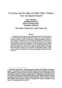


![[PDF BOOK] Foundations of Financial Management with Time Value of ...](https://p.pdfkul.com/img/300x300/pdf-book-foundations-of-financial-management-with-_5a2fcab91723dd8d968d9783.jpg)


