Using Stochastic NTCC to Model Biological Systems Carlos Olarte and Camilo Rueda Javeriana University, Dept. Computer Science. Cali, Colombia {caolarte,crueda}@atlas.puj.edu.co Abstract Concurrent process calculi are powerful formalisms for modeling concurrent systems. The mathematical style underlying process calculi allow to both model and verify properties of a system, thus providing a concrete design methodology for complex systems. ntcc , a constraints-based calculus for modeling temporal nondeterministic and asynchronous behavior of processes has been proposed recently. Process interactions in ntcc can be determined by partial information (i.e. constraints) accumulated in a global store. ntcc has also an associated temporal logic with a proof system that can be conveniently used to formally verify temporal properties of processes. We are interested in using ntcc to model the activity of genes in biological systems. In order to account for issues such as the basal rate of reactions or binding affinities of molecular components, we believe that stochastic features must be added to the calculus. In this paper we propose an extension of ntcc with various stochastic constructs. We describe the syntax and semantics of this extension together with the new temporal logic and proof system associated with it. We show the relevance of the added features by modeling a non trivial biological system: the gene expression mechanisms of the λ virus. We argue that this model is both more elaborate and compact than the stochastic π calculus model proposed recently for the same system. Keywords: NTCC, Lambda-Switch, biological systems, concurrent process calculus, concurrent constraint programming Resumen Los c´ alculos de procesos concurrentes son un poderoso formalismo para modelar sistemas concurrentes. El soporte matem´ atico del c´ alculo permite modelar y probar propiedades de un sistema, proveyendo as´ı, una metodolog´ıa concreta para el dise˜ no de sistemas complejos. ntcc es un c´ alculo basado en restricciones propuesto recientemente para modelar comportamiento no determin´ıstico y as´ıncrono. La interacci´ on de los procesos en este c´ alculo es determinada por medio de informaci´ on parcial (es decir restricciones) acumuladas en un almac´en global de restricciones. Adicionalmente, ntcc cuenta con una l´ ogica temporal y un sistema de inferencia que puede ser utilizado para verificar formalmente propiedades de los procesos. Nosotros estamos interesados en utilizar ntcc para modelar el comportamiento de los genes en los sistemas biol´ ogicos. Sin embargo, para ello se hace necesario la introducci´ on de caracter´ısticas estoc´ asticas en el c´ alculo para modelar por ejemplo la afinidad entre las mol´eculas. En este art´ıculo proponemos una extensi´ on de ntcc con algunos operadores estoc´ asticos. Para dicha extensi´ on describimos la sintaxis , la sem´ antica y una nueva l´ ogica temporal junto con su sistema de inferencia. A partir de este, modelamos el mecanismo de expresi´ on de los genes del virus λ y mostramos que dicho modelo es mas simple y compacto que el modelo propuesto recientemente utilizando el c´ alculo π estoc´ astico. Palabras claves: NTCC, Lambda-Switch, Sistemas biol´ ogicos, C´ alculos de procesos concurrentes, Programaci´ on concurrente por restricciones
1
Introduction
We are interested in using soft computing techniques for modeling complex systems such as those arising frequently in biology. From a broad perspective we view soft computing as those techniques pertaining to systems that can best be described as a collection of processes dealing with partial information. What
”partial” means depends on the particular application. It can refer to being able to use partial knowledge of a state of affairs and to perform different kinds of guessing (bounded or unbounded non determinism, probabilistic choices, approximate answers). In this view, concurrency also belongs to this realm since it deals with partial information on the ordering of events. So does constraint programming which is based on the very idea of computing with predicates expressing different degrees of knowledge about variable values. Concurrent constraint (CC) process calculi [11] provides formal grounds to the integration of concurrency and constraints so that non trivial properties of concurrent systems can be expressed and proved. They are thus natural simulators to gain experience on different soft computing techniques. We view biological phenomena at the molecular level as constructed from very complex interactions among a great number of concurrent processes acting at different biological scales. Concurrent processes occurring in molecular biology exhibit a rich variety of synchronization schemes, calling into play different degrees of precision (i.e. partial information) about temporal or chemical relations involving them. The complexity of biological phenomena poses a great challenge to any computational formalism. We think that a suitable CC process calculus should provide a convenient framework to get insights into the right models to cope with this challenge. We thus borrow concepts and techniques from concurrent processes modeling to define suitable computational calculi and analyze their behavior in real biological settings. What we gain from this low level approach is twofold. On the one hand, we are able to ground the development of simulation tools on a very precise formal foundation and by this means proposing coherent models of higher level biological structures and operations. On the other hand, our model can give us clues for constructing formal proofs of interesting properties of a given biological process. We propose using a temporal non deterministic concurrent calculus (ntcc , see [6]) as a formal base to model timed gene activity processes in such a way that their biological properties can be formally proved. This goes in the same direction as the concurrent process calculi models of biological systems proposed recently ([9], [2], [3]). The ntcc calculus inherits ideas from the tcc model [10], a formalism for reactive concurrent constraint programming. In tcc time is conceptually divided into discrete intervals (or time-units). In a particular time interval, a deterministic ccp process receives a stimulus (i.e. a constraint) from the environment, it executes with this stimulus as the initial store, and when it reaches its resting point, it responds to the environment with the resulting store. Also the resting point determines a residual process, which is then executed in the next time interval. The ntcc calculus is obtained from tcc by adding guarded-choice for modeling non-determinism and an unbounded but finite delay operator for asynchrony. Computation in ntcc progresses as in tcc, except for the non-determinism and asynchrony induced by the new constructs. The calculus allows for the specification of temporal properties, and for modeling and expressing constraints upon the environment both of which are useful in proving properties of timed systems. However, ntcc does not provide stochastic constructs. These are fundamental to faithfully model aspects such as the effect of reactions on concentration of particular components, affinities or distances. We thus propose orthogonal extensions of ntcc to account for the stochastic behavior of processes. In this paper we are interested in showing how non trivial biological processes calling into action different forms of partial information can be modeled in ntcc extended with suitable stochastic constructs. We also investigate ways in which properties of a biological process can be formally proved. We are able to do this thanks to the logical nature of ntcc, which comes to the surface when we consider its relation with linear temporal logic: All the operators of ntcc correspond to temporal logic constructs. Since we extend ntcc , new linear temporal logic and proof system must also be provided. We propose both and use them to prove some properties of a gene regulation system called the lambda switch. Our model using the stochastic extension is both simpler and more complete than the one recently proposed in [3]. The main contributions of this paper are: 1) to define an orthogonal extension adding stochastic constructs to ntcc , 2) to couple the extended calculus with a suitable temporal logic and proof system, 3) to show how the expressiveness of the extended ntcc model allows faithful and simple descriptions of complex systems of interacting biological processes, such as the lambda switch and 4) showing that by modeling a gene activities system in the extended stochastic ntcc one inherits a well defined logical inference system (also proposed here) that can be used to prove interesting temporal properties (or lack thereof) of the system.
2
2
Background
2.1
NTCC Calculus
In concurrent constraint calculi such as ntcc, process interactions can be determined by partial information (i.e. constraints) accumulated in a global store. The particular type of constraints is not fixed but specified in a constraint system that is considered a parameter of the calculus. 2.1.1
Constraint System
A constraint represents a piece of partial information over a set of variables. For example, in constraint x > 3, the value of x is unknown but we can assert that it is greater than 3. A constraint system provides a signature from which constraints can be constructed. It also provides an entailment relation (|=) over constraints where c1 |= c2 holds iff the information of c2 can be inferred from c1 . P P Formally, a constraint system is a tuple h , ∆i where is a signature (i.e a set of constants, functions and P P predicate symbols) and ∆ is a consistent first-order theory over (i.e P a set of sentences over having at least one model). Constraints can be viewed as first-order formulae over and c |= d holds if the implication c ⇒ d is valid in ∆ [6]. For practical reasons the entailment relation must be decidable. A constraint store is a a set of variables and a conjunction of formulae (i.e constrains) between them. It is used to share information between process and for synchronization purposes. The store is monotonically refined by adding information using tell operations of the calculus. For example, tell(x < 2) adds constraint x < 2 to the store. Additionally, we can test if a constraint c can be entailed from the store by means of ask operations. For example, ask(x < 5) tests whether store |= x < 5. The ask operation blocks when neither store |= x < 5 nor store |= ¬(x < 5) holds. 2.1.2
Overview
ntcc [6] is a process calculus that extends tcc [10]. In both of them, processes share a common store of partial information [11]. Both ntcc and tcc have an explicit notion of (discrete) time. ntcc time is conceptually divided into discrete intervals (or time-units). In a particular time interval, a deterministic ccp process receives a stimulus (i.e. a constraint) from the environment, it executes with this stimulus as the initial store, and when it reaches its resting point, it responds to the environment with the resulting store. Also the resting point determines a residual process, which is then executed in the next time interval. ntcc has been successfully used to model many real life system such as reactive system, robot behavior [5] and music composition [6]. Unlike tcc, ntcc includes constructs for modeling nondeterminism and asynchrony. A very important benefit of being able to specify non-deterministic and asynchronous behavior arises when modeling the interaction among several components running in parallel, in which one component is part of the environment of the others. This is frequent in biological settings. These systems often need non-determinism and asynchrony to be modeled faithfully.
2.1.3
Process Syntax
In this section we describe briefly the syntax of ntcc processes. See [6] for further details. ntcc provides the following constructors: def
• tell : adds new information to the constraints store. For example, the process P 1 ≡ tell (c > 5) adds constraint c > 5 to the store. P • i∈1..n when ci do Pi chooses non-deterministically a process Pi whose guard ci is entailed by the def
store. For example, process P2 ≡ when (c < 3) do tell (d = 5) + when (e > 5) do tell (d < 3) adds the information d = 5 when constraint c < 3 is entailed from the current store. On the other hand, if e > 5 is entailed, d < 3 is asserted. When both guards are entailed a non-deterministic choice is performed.
3
• Given two ntcc processes P and Q, process P ||Q represents the parallel composition between P and Q. • local x in P behaves like P but the information of the variable x is local to P , i.e. P cannot see information about a global variable x and processes which are not part of P cannot see the information generated by P about x. • next P executes process P in the next time unit (unit-delay) • unless c next P executes P iff c cannot be entailed by the constraint store in the current time unit • !P executes P in all time units from the current one on. It can be viewed as P ||next P ||next next P ||... • ?P represents unbounded but finite delays, i.e P eventually will be executed. This process can be viewed as P + next P + next next P...next n P where n is a finite natural number. Two new operators (ρP and ?ρ P ) will be introduced in section 3.1 to express stochastic behavior. They will be illustrated in the model of the lambda switch. 2.1.4
Rules of internal reduction
In this section we show the operational semantics of ntcc by giving reduction rules for each process. These rules will help us to understand how ntcc processes interact with each other until they reach a quiescent point. Recall that when this state is reached, another time units is created with an empty constraint store and the residual process. For a complete description of ntcc semantics refer to [6]. Reduction rules are based on configurations. A configuration hP, di is composed of a ntcc process P and a store d. For tell processes we have: T ELL
htell c, di → hskip, d ∧ ci
where skip is the empty process. This reaction says that a tell process adds information (a constraint) to the constraint store d. In when c do P processes the rule is as follows: SU M P if d |= cj , j ∈ I h i∈I when ci do Pi , di → hPj , d ∧ ci It means that a particular process Pj is non-deterministically chosen for execution among all those whose guard (ci ) can be entailed from the current store d. For parallel composition we have: hP, ci → hP 0 , di P AR hP ||Q, ci → hP 0 ||Q, di It says that if P evolves to P 0 , then the same transition can occur if we execute P in parallel with some process Q. Parallel composition is commutative. For unless c next P processes: U N LESS
hunless c next P, di → hskip, di
if d |= c
The rule says that nothing is done when c is entailed by the store. Finally, the rule for star processes is: ST AR
h?P, di → hnext n P, di
if n ≥ 0
It means that process P will be run in the (undetermined) future. The above rules define so-called internal transitions. In addition to these, ntcc defines an observable transition which is the one that goes from one time unit to the next. At the end of a time unit the resulting store can be observed by the environment. Then, processes contained in next constructs are scheduled for the next time unit. This include those defined by unless processes whose guard cannot be entailed from the current store (see [6] for details). 4
2.2
Linear-temporal Logic in ntcc
ntcc can be used to verify properties over timed systems. It provides for this a linear temporal logic in which temporal properties over infinite sequences of constraints can be stated [6]. The syntax of this logic is as follows: · · · A, B, ... : c | A ⇒ A | ¬A | ∃x A | ◦ A | ♦A | �A ·
·
·
c is a constraint. ⇒, ¬ and ∃x represent the linear-temporal logic implication, negation and existential quantification, respectively [4]. These symbols should not be confused with their counterpart in the constraint system (i.e ⇒ , ¬ and ∃). Symbols ◦ , � and ♦ denote the temporal operators next, always and eventually. The interpretation structures of formulae in this logic are infinite sequences of states [4]. In ntcc , states are replaced by constraints. Given the set C of constraints in the constraint system, let α ∈ C ∞ be an infinite sequence of constraint and α(i) the i − th element of α. We say that α ∈ C ∞ is a model of (or that ii satisfies) A, notation α |= A, if hα , 1i |= A where: hα hα hα hα hα hα
, , , , , ,
ii |= c · ii |= ¬A · ii |= A1 ⇒ A2 ii |= ◦A ii |= �A ii |= ♦A
if f if f if f if f if f if f
α(i) |= c hα , ii |= \ A hα , ii |= A1 implieshα , ii |= A2 hα , i + 1i |= A ∀j≥i hα , ji |= A ∃j≥i s.t.hα , ji |= A
if f
there is an x − variant α0 of α s.t. hα0 , ii |= A
·
hα , ii |= ∃x A
(1)
In the last expression, d and α0 are x−variants of c and α , respectively, if they are the same except for the information about x. In [6] a proof system is built on the top of this logic. Given a process P and a formula A, a proof of P |= A can be obtained by following a set of inference rules. Nevertheless, we are interested in proving properties with probabilistic statements such as “The concentration of component c will eventually become 0 with probability ρ”. In section 3.3 we provide an inference system to prove these kind of properties. 2.3
Lambda Switch
In this section we give a brief description of a biological system (called the λ switch) that we model in section 4 using our proposed extension of ntcc . For additional details see [3] or [1]. Bacteriophage λ is a virus that infects the Escherichia coli bacterium. As we will see, this biological system exhibits cooperativity relationships and non-deterministic behavior. When the virus injects its genome into the bacteria, there are two states that the bacteria can reach: (1)lytic growth in which the virus produces new viruses and (2) lysogeny in which the viral genome is passed to new generations in a passive way. The switching between states is determined by processes in a region of the virus genome called the λ switch (see figure 1). In this switch there are two promoter regions called P RM and P R where production of rep and cro proteins, respectively, take place. The lytic growth state is characterized by a high concentration of cro proteins whereas lysogeny is characterized by a high concentration of rep. Promoters are overlapped by three regions (binding sites) called OR1, OR2 and OR3. Region OR1 exhibits a high affinity for rep and a low affinity for cro. On the other hand, OR3 exhibits a high affinity for cro and a low affinity for rep. In lysogeny, rep proteins usually bind OR1 and OR2. When OR1 is bound by rep, OR2 affinity for rep increases. This is a cooperation relation between bindings at different sites. On the other hand, OR3 and the promoter P RM are usually vacant but eventually bound by the polymerase RN AP . When this occurs, the transcription of the gene cI starts and new instances of rep proteins are produced. When OR1 is not vacant, binding of RN AP to P R is inhibited, stopping in this way the production of cro. Another cooperation relationship is present in the lambda switch: since P RM is a weak promoter, when OR2 is bound by rep, rep cooperates with RN AP and more frequent transcriptions of gene cI happen. It implies that more rep 5
(a) Lytic growth
(b) Lysogeny
Figure 1: Lambda switch states proteins are produced thus increasing the chance of maintaining the lysogeny state. Lysogeny state is maintained until an environmental signal turns the switch to the lytic growth. This process is called Induction and it occurs with very low probability. In this state the concentration of rep decreases dramatically and so RN AP has the chance to bind to OR1, that is now vacant most of the time. P R, a stronger promoter than P RM , starts the transcription of gene cro and thus new instances of cro are produced. Because OR3 has a high affinity for cro, it is bound by this protein avoiding RN AP bindings to P RM . This biological system has been successfully modeled in [3] by using the π calculus [8] with stochastic behavior [7]. However, we believe that notions such as cooperation and the effect of distance (i.e reactions may occur depending on the distance between molecules) can be expressed in a more straightforward manner by using the notion of constraint. We also introduce some additional details that were left aside in the model in [3].
3
Introducing Stochastic Behavior in ntcc
In this section we introduce two new operators in ntcc for modeling stochastic behavior. We also propose an extension of the ntcc linear-temporal logic that can be used to prove properties involving probabilistic statements. 3.1
?ρ P Processes
Star processes are used to express eventually in ntcc . However, we should be able to differentiate between two processes that eventually occur with different probabilities. For example, the induction process in the lambda switch occurs eventually but with a very low probability, while bindings between rep and region OR3 are quite frequent in lysogeny. We propose the constructor ?ρ P in which P eventually occurs with probability ρ. Operationally: ST ARρ
h?ρ P, di → hnextn P, di
if n ≥ 0 ∧ Φ(ρ) = 1
where Φ : < ∈ [0, 1] → bool. Φ can be computed by generating pseudo-random numbers following a binomial distribution with probability ρ and 1 as number of events. If Φ(ρ) = 1 we say that the process will be executed, otherwise it will not. This operator can be expressed as combinations of the original ones: def
?ρ P ≡ local x in ? (tell x = Φ(ρ)||when x = 1 do P ) by adding the function Φ to the signature of the constraint system.
6
ρP
3.2
The previous constructor operates over an arbitrary time interval. We are interested in expressing processes that occur in a single time unit but with a probability ρ. Those processes, denoted ρ P , can be expresses as follows: (2) ρ P ≡ local x in tell (x = Φ(ρ))||when x = 1 do P Operationally: RHOP 3.3
hρ P, di → hP, di
if Φ(ρ) = 1
Stochastic parameters in the linear-temporal logic
To prove properties such as “The concentration of rep will eventually become 0 with probability ρ” we change the structure of formulae by adding probabilities, i.e formulae will be tuples hA , ρi where A is a formula in the ntcc lineal-temporal logic. The new operators are as follows: ◦
◦
◦
A0 , B 0 , .... = hc, ρi | A0 ⇒ A0 | ¬A0 | ∃x A0 | ◦ A0 , | ♦A0 | ♦A0 Probability ρ should not be confused with some notion of degree of validity of the formula. This probability refers to the occurrence of events (time). For example, the formula hc < 3, 0.5i expresses that with a probability of 0.5 constraint c < 3 will be asserted. The semantics of our new logic is as follows: hα hα hα hα hα hα
, , , , , ,
ii |= hc , ρi ◦ ii |= ¬hA , ρi ◦ ii |= hA1 , ρ1 i ⇒ hA2 , ρ2 i ii |= ◦hA , ρi ii |= �hA , ρi ii |= ♦hA , ρi
if f if f if f if f if f if f
α(i) |= hc , ρi hα , ii |= \ hA , 1 − ρi hα , ii |= hA1 , ρ1 i implieshα , ii |= hA2 , ρ2 i hα , i + 1i |= hA , ρi ∀j≥i hα , ji |= hA , ρi ∃j≥i s.t.hα , ji |= hA , ρi
if f
there is an x − variant α0 of α s.t. hα0 , ii |= hA , ρi
◦
hα , ii |= ∃x hA , ρi
(3)
where α(i) |= hc , ρi is defined as: hc1 , ρ1 i |= hc2 , ρ2 i iff c1 entails c2 in the constraint system and ρ2 ≤ ρ 1 . 3.3.1
Inference System
We extend the inference system proposed in [6] with inferences rules taking into account the new form of formulae and the probabilistic operators ρ P and ?ρ P . The rules are as follows: LT ELL : tell c ` hc , 1.0i LP AR :
(4)
P ` hA , ρi Q ` hB , ρ2 i ◦
P ||Q ` hA , ρi ∧ hB , ρ2 i
(5)
i.e. the parallel execution of two process satisfies the conjunction of the formulae of each process. LLOC :
P ` hA , ρi ◦
local x in P ` ∃x hA , ρi
LN EXT : LU N L :
P ` hA , ρi next P ` ◦hA , ρi P ` hA , ρi ◦
unless c next P ` hc , 1.0i ∨ ◦hA , ρi
LCON S :
P ` hA , ρi ◦ if hA , ρi ⇒ hB , ρ2 i P ` hB , ρ2 i 7
(6) (7) (8) (9)
LST AR :
P ` hA , ρi ?P ` ♦hA , ρi
(10)
∀i ∈ I Pi ` hAi , ρi i ◦ ◦ W ◦ ◦ V ◦ i∈I when ci do Pi ` i∈I (hci , 1i ∧ hAi , ρi i) ∨ i∈I ¬hc1 , 1.0i
LSU M : P
P P RO :
P ` hA , ρi P ` hA , ρ × ρ2 i ρ2
(11)
(12)
The previous equation represents the inference rule for ρP processes. Since the probability ρ and the probability ρ2 are independent, the probability of both occurrences is ρ × ρ2 . Finally, the rule for the ?ρ P process is: P ST AR :
4
P ` hA , ρi ?ρ2 P ` ♦hA , ρ × ρ2 i
(13)
Modeling the λ-Switch with the stochastic ntcc extension
Recall that our objective is to use concurrent calculi to faithfully model biological systems. We test the appropriateness for this task by constructing a (somewhat) detailed model of the lambda-switch using the def
extended calculus defined above. We use process definition constructs of the form PROCESS(x) ≡ P that do not formally belong to the calculus. These, however, can be easily defined in terms of the standard calculus constructs (see [6]). 4.1
REP and CRO Protein Control
In our model production of rep proteins is controlled by 3 extended calculus processes: (1) Induction, that reduces the concentration of rep thus switching the system to a lytic growth state, (2) a process supervising that the concentration of rep does not exceed a given threshold and (3) a process that increases the concentration of rep as a result of the expression of gene cI. The induction process (see section 2.3), activated by environment signals that are at present little understood, causes a strong reduction of rep proteins and therefore switching to a lytic growth state. The occurrence probability for this process is very low. By using ?ρ P processes we can model this fact as: def
INDUCTION(ρind ) ≡ ?ρind (tell reset repc )
(14)
Eventually, under the probability ρind , this process reduces the concentration of rep to 0 (see reset repc in equation 21). The following process avoids a negative feedback by controlling the concentration of rep proteins. This represents the situation in which there are so many rep proteins floating around that even OR3 will get bound to rep thus inhibiting gene cI expression. The process inhibits the production of rep when concentration reaches repthreshold . def
REPTHOLD(repthreshold ) ≡ when Crep > repthreshold do next tell inhibitrep 4.2
(15)
Gene transcription
As mentioned before, P RM is a weaker promoter than P R . This means that production of rep takes more time than production of cro once RN AP binds to P RM (resp. P R ). Sometimes no rep protein is produced at all when the binding occurs, i.e RN AP falls off without transcribing gene cI. We model the gene transcription at the P R promoter as follows: def
CROtrans ≡ when prbound do
8
ρcrotrans (tell
inc croc )
(16)
where predicate prbound is true iff RN AP is binding P R . Constraint inc croc causes a new (higher) value for concentration of cro proteins to be asserted in the next time unit ( see equation 21). Modeling gene transcription at P RM is more difficult because the probability of transcription may vary according to the presence or absence of rep at OR2 . When OR2 is bound by rep , the probability of gene cI transcription at P RM is higher and in consequence higher is also the probability of producing more reps. Equation 17 models gene transcription at P RM : def
CItrans(ρhigh , ρlow ) ≡ when ¬inhibitrep ∧ prmbound do local p in (when or2 bound rep do tell p = ρhigh (17) + when or2 bound cro ∨ or2 vacant do p = ρlow ) || p (tell inc repc ) where cooperativity is modelled by means a when c do P process that chooses between ρ high and ρlow in order to execute tell inc(repc ) with the right probability. Notice that synchronization is guaranteed by the use of constraints: process p (tell inc repc ) blocks until the value of p is known. 4.3
Operator Regions
In what follows we model the behavior of the OR1, OR2 y OR3 binding sites. Since each operator has different affinities for rep and cro , ρ P type processes are needed. OR2 and OR1 exhibit another cooperativity relationship: OR2 increases its affinity for rep when OR1 is bound by rep . The following equations model the operator regions in the lambda switch: def
OR1 ≡ when or1 unbound do when repc > 0 do ρor1rep (next tell (or1 rep bound ∧ dec repc )) + when croc > 0 do ρor1cro (next tell (or1 cro bound ∧ dec croc )) when or1 rep bound do 1.0−ρor1rep (next tell (or1 unbound ∧ inc repc )) + when or1 cro bound do 1.0−ρor1cro (next tell (or1 unbound ∧ inc croc ))
(18)
def
OR2 ≡ local or2rep in when or2 unbound do when repc > 0 do ρor2rep (next tell (or2 rep bound ∧ dec repc )) + when croc > 0 do ρor2cro (next tell (or2 cro bound ∧ dec croc )) + when ¬or1 bound rep do tell (ρor2rep = ρor2rep low) when or2 rep bound do 1.0−ρor2rep (next tell (or2 unbound ∧ inc repc )) when or2 cro bound do 1.0−ρor2cro (next tell (or2 unbound ∧ inc croc )) k(when or1 bound rep do tell (ρor2rep = ρor2rep high)
(19)
def
OR3 ≡ when or3 unbound do when repc > 0 do ρor3rep (next tell (or3 rep bound ∧ dec(repc )) + when croc > 0 do ρor3cro (next tell (or3 cro bound ∧ dec(croc )) when or1 rep bound do 1.0−ρor3rep (next tell (or3 unbound ∧ inc(repc )) + when or1 cro bound do 1.0−ρor3cro (next tell (or3 unbound ∧ inc(croc ))
(20)
where ρor1rep,ρor1cro,ρor2rep high,ρor2rep low,ρor3rep and ρor3cro are the probabilities (affinities) of each binding site w.r.t rep and cro. Constraints dec repc and dec croc will cause decrementing of the concentration of rep (resp. cro ) in the environment (see equation 21). In the above processes, when the operator is unbound (i.e vacant) and reps or cros are available in the environment, eventually the protein (i.e rep or cro) binds the operator and consequently also decreases the protein concentration in the environment. Finally, equation 21 controls the concentration of rep and cro for the next time unit: def
CONCCTR ≡ (when reset repc do next tell repc = 0 + when inc repc ∧ ¬reset repc do next tell (repc = repc + 1)+ when dec repc ∧ ¬reset repc do next tell (repc = repc − 1))|| (when inc croc do next tell (croc = croc + 1) + when dec croc do next tell (croc = croc − 1)) (21) 9
4.4
RNAP binding
Equations 16 and 17 depend on bindings between RN AP and promoters P R and P RM , respectively. The behavior of RN AP has two components: (1) when RN AP is binding P R (resp P RM ), there is a probability of 1.0 − ρrnap pr (resp. 1.0 − ρrnap prm) of falling off thus interrupting gene transcription. And (2) when promoters are unbound, RN AP may bind to P R (resp P RM ) if OR1 (resp. OR3) is vacant, with probability rnap pr (resp. rnap prm). Equation 22 models this fact: def
RNAPCTR ≡ when rnap unbound do ( when or1 unbound do rnap pr (next tell (or1 rnap bound ∧ pr bound)) + when or3 unbound do rnap prm (next tell (or3 rnap bound ∧ prm bound)) +when rnap bound do ( when or1 rnap bound do 1.0−rnap pr (next tell or1 unbound) +when or3 rnap bound do 1.0−rnap prm (next tell or3 unbound))
(22)
With equations 14 to 22 we can describe the overall lambda-switch system as follows: λ − PROC(ρ ind, rep thr, ρor1rep, ρor2rep high, ρor2rep low, ρor3rep, def
ρor1cro, ρor2cro, ρor3cro, ρcrotrans, ρcitrans high, ρcitrans low) ≡ local repc (0), croc (0), prbound , prmbound inhibitrep or1 bound rep, or1 bound cro, or2 bound rep, or2 bound cro, or2 bound rep, or2 bound cro, or1 unbound, or2 unbound, or3 unbound, rnap bound, rnap unbound, or1 bound rnap, or2 bound rnap, or3 bound rnap ρor1rep , ρor2rep , ρor3rep , ρor1cro, ρor2cro , ρor3cro in IN DU CT ION (ρ ind)||!REP T HOLD(rep thr)||!CROtrans||!CItrans|| !OR1||!OR2||!OR3||!RN AP CT R||!CON CCT R
(23)
This equation defines the stochastic parameters of the model and then execute concurrently the processes needed to control the behavior of the lambda switch. 4.5
Proving temporal properties of the λ switch system
In this section we show proofs for two properties the lambda switch system must satisfy: • Eventually, with probability ρ (a very low probability in this case) the concentration of rep proteins drops to zero . • If OR1 and OR2 are bound by reps and OR3 is bound by RN AP , a new instance of rep will eventually be produced (i.e. the protein concentration will be incremented) with probability ρ ci high . Recall that when OR2 is bound by rep, the rate of transcription of gene cI is incremented because of the cooperativity relationship between OR2 and P RM . In order to proof the first property, we star with the definition of the overall system: LP AR :
IN DU CT ION ` hA , ρi OR1 ` hA2 , ρ2 i ... RN AP CT R ` hAn , ρn i ◦
◦
λ − P ROC ` hA , ρi ∧ �hA2 , ρ2 i...� ∧ hAn , ρn i
(24)
Notice that we use the temporal always operator because processes are replicated (i.e. use the “!” prefix) in the definition of λ − P ROC. By using LCON S in equation 24 we get: LP AR : λ − P ROC ` hA , ρi
(25)
The IN DU CT ION process satisfies the formula hA , ρi. Now, we are going to find out the structure of A:
10
P ST AR :
tell reset(repc ) ` hreset(repc ) , 1.0i ?ρ ind tell reset(repc )||IN DU CT ION ` ♦hreset(repc ) , ρ indi
(26)
def
As IN DU CT ION ≡ ?ρ ind tell reset(repc )||IN DU CT ION (omitting the local hiding), we can affirm that λ − P ROC satisfies the property “eventually under a probability ρ ind the concentration of rep will be zero” , i.e, ♦hreset(repc ) , ρ indi. To prove the second property we star from the definition of λ − P ROC and then use the definitions of CItrans and RN AP CT R: LP AR :
RN AP CT R ` hA , ρi
CIT RAN S ` hA2 , ρ2 i ... ◦
λ − P ROC ` �hA , ρi ∧ �hA2 , ρ2 i...
(27)
Using the definition of CIT RAN S we get: tell p = ρ high ` hp = ρ high , 1.0i
tell p = ρ low ` hp = ρ low , 1.0i
tell p = ρ high + when or2 vacant do tell p = ρ low ` LSU M : when or2 bound rep do · ◦ · ◦ hor2 bound rep ∧ p = ρ high , 1.0i ∨ hor2 vacant ∧ p = ρ low , 1.0i∨
(28)
· ·
·
h¬or2 bound rep ∧ ¬or2 vacant , 1.0i ·
·
Since the premise is the formula hor1 bound rep ∧ or2 bound rep ∧ or3 bound rnap , 1.0i we can use LCON S as follows: ·
·
hor1 bound rep ∧ or2 bound rep ∧ or3 bound rnap , 1.0i LCON S : when or2 bound rep do tell p = ρ high + when or2 vacant do tell p = ρ low ` hp = ρ high , 1.0i
(29)
Finally, by using P P RO we can verify that CIT RAN S satisfies the following formula: when or2 bound rep do tell p = ρ high + when or2 vacant do tell p = ρ low ` hp = ρ high , 1.0i when ... do ... + when ... do ...|| p high(tell inc(repc )) ` hinc(repc ) , ρ highi (30) Equation 30 says that new reps will appear with a probability ρ high verifying the cooperative behavior between OR2 and P R .
5
Concluding remarks and Future Work
We have given orthogonal extensions of ntcc for modeling stochastic behavior of processes. In particular, we proposed two new operators: ?ρ P and ρ P . The first one expresses that P is eventually executed with probability ρ and the second one that P is executed in the current time unit with probability ρ. We showed that both can be expressed in terms of existing ntcc constructs by including in the signature of the underlying constraint system of ntcc a probabilistic function Φ(ρ) : [0, 1] → bool following a binomial distribution. The syntax and semantics associated to the temporal logic and proof system of ntcc were modified accordingly to account for the new stochastic constructs. We have shown that the proposed extension provides enough expressiveness to faithfully model a non trivial stochastic system. Using this new stochastic non-deterministic calculus we were able to provide a model of a biological system called the lambda switch that is both simpler and more complete than models previously proposed based on the stochastic π-calculus. Finally, an inference system to prove probabilistic properties in the calculus was provided. This inference system is built on an ntcc linear-temporal logic extension by adding probabilities to each formula. For each process construction including our new processes ?ρ P and ρ P , we defined an inference rule to proof if a process P satisfies an specification (i.e a formula in the logic). We showed the use of this system by proving two properties in our lambda switch model. 11
In the short term we plan to implement a ntcc stochastic processes simulator to better visualize process behavior. We will build it up from a ntcc framework previously developed by our group ([5]) . This will allow us to trace the evolution of protein concentrations so as to assess our model w.r.t. existing biological data for the lambda switch. Additionally, we expect to use our proof system to verify properties of relevance to biologists. Adapting or implementing a new automatic theorem-prover will help us in this task. We also plan to construct reasonably complete models of some other biological systems such as the N A pump [2].
References [1] Adam Arkin, John Rossb, and Harley H. McAdams. Stochastic kinetic analysis of developmental pathway bifurcation in phage lambda-infected escherichia coli cells. In Genetics, 1998. [2] D. Besozzi and G. Ciobanu. A p system description of the sodium-potassium pump. In Workshop on Membrane Computing, 2004. [3] Celine Kuttler, Joachim Niehren, and Ralf Blossey. Gene regulation in the pi calculus: Simulating cooperativity at the lambda switch. In Bio-CONCUR 2004, 2004. [4] Z. Manna and A. Penueli. The Temporal Logic of Reactive and Concurrent Systems, Sepecification. Springer, 1991. [5] Pilar Munoz and Andres Hurtado. Programming robot devices with a timed concurrent constraint programming. In Principles and Practice of Constraint Programming - CP2004. LNCS 3258, page 803. Springer, 2004. [6] Mogens Nielsen, Catuscia Palamidessi, and Frank D. Valencia. Temporal concurrent constraint programming: Denotation, logic and applications. In Special Issue of Selected Papers from EXPRESS’01, Nordic Journal of Computing, 2001. [7] C. Priami. Stochastic pi-calculus. In Computer Journal, 2004. [8] J. Parrow R. Milner and D. Walker. A calculus of mobile processes, Parts I and II. Journal of Information and Computation, 100:1–77, September 1992. [9] Aviv Regev, William Silverman, and Ehud Y. Shapiro. Representation and simulation of biochemical processes using the pi-calculus process algebra. In Pacific Symposium on Biocomputing, pages 459–470, 2001. [10] V. Saraswat, R. Jagadeesan, and V. Gupta. Fundation of timed concurrent constraint programming. In IEEE Symposium on Logic in Computer Science. IEEE press, 1994. [11] V. A. Saraswat. Concurrent Constraint Programming. The MIT Press, Cambridge, MA, 1993.
12