Where Should We Build a Mall? The Formation of Market Structure and Its Effect on Sales* Doug J. Chung, Harvard University Kyoungwon Seo, Seoul National University Reo Song, California State University, Long Beach
July, 2017 Abstract We estimate a structural model that takes into account the entry decisions of retail stores and their corollary effects on total shopping mall sales. By understanding the endogenous behavior of individual store entry, we provide guidance on location choice for mall developers. We find negative competition effects to dominate within store categories—especially among discount and midscale stores—but positive agglomeration effects to exist across store categories. Although varying by store brand, our results suggest that upscale stores are likely to enter malls in more populated, affluent areas, whereas midscale stores enter less populated, lower-income areas. We find positive causal brand effects for specific upscale and midscale stores, above and beyond market effects, but find negative causal brand effects for all discount stores on mall sales. This paper also introduces three main methodological innovations to the marketing literature. First, we correct for endogeneity with regard to both store entry and mall sales to identify the causal effect of store entry on mall sales. Second, we address multiple equilibria by estimating equilibrium selection from the observed data. Finally, we overcome the computational burden of solving games of complete information with multiple equilibria by utilizing the GPGPU technology, using multiple processing cores in a graphics processing unit to noticeably increase computational speed. Key words: firm entry, discrete game, complete information, multiple equilibria, endogeneity, GPGPU technology, Bayesian estimation, shopping mall, spillover.
*
Comments are welcome to Kyoungwon Seo, Seoul National University, Seoul, South Korea, [email protected]. The authors thank Jose Alvarez, Jinhee Jo, the seminar participants at HKUST, and the conference participants at the 2016 Marketing Science Conference for their comments and suggestions. The authors also thank Harvard Business School, and the Institute of Finance and Banking and Management Research Center at Seoul National University for providing financial support.
1. Introduction The retail sector constitutes one of the largest segments of the U.S. economy, generating sizeable annual sales that considerably bolster total GDP. In 2015, retail sales totaled $4.7 trillion in the U.S. alone (approximately 26 percent of GDP) and nearly $21 trillion globally1, and the market continues to grow. Retail is the largest private employer in the United States, directly and indirectly contributing 42 million jobs, or one in four.2 Despite the recent e-tail surge, traditional brick-and-mortar stores still remain the core of the retail industry. In 2015, U.S. retail e-commerce sales accounted for only 7.3% of total U.S. retail sales. Furthermore, according to a recent survey of over 1,000 consumers, more than 70% would prefer to shop at a brick-and-mortar Amazon store versus Amazon.com, and 92% of millennials planned to shop in-store in 2015 as often or more than they did in 2014.3 A considerable proportion of brick-and-mortar retail in both developed countries, such as the United States, and newly industrialized countries, such as China, involve a market structure typically referred to as a shopping mall or a shopping center. According to government statistics, China’s retail sales have more than quadrupled in a 10year span from 6.7 trillion yuan in 2005 to 30 trillion yuan in 20154, creating one of the world’s largest consumer markets. In fact, analysts estimate that in 2016 China will surpass the U.S. as the world’s largest retail market. 5 In an effort to keep up with this explosive increase in consumption, global shopping-center development is increasing rapidly. According to a CBRE report, 39 million square meters of new mall space worldwide was under construction in 2015, with
1
Worldwide Retail Ecommerce Sales: The eMarketer Forecast for 2016, http://totalaccess.emarketer.com/Reports/Viewer.aspx?R=2001849&dsNav=Ntk:basic%7cglobal+retail+sales%7c1%7c, Ro:4,Nr:NOT(Type%3aComparative+Estimate). 2 National Retail Federation, “The Economic Impact of The U.S. Retail Industry”, https://nrf.com/resources/retail-library/the-economic-impact-of-the-us-retail-industry 3 Timetrade.com, May 18, 2015, “Study: 85% of Consumers Prefer to Shop at Physical Stores vs. Online”, http://www.timetrade.com/news/press-releases/study-85-consumers-prefer-shop-physical-stores-vs-online. 4 National Bureau of Statistics of China, “Total Retail Sales of Consumer Goods in December 2015”, January 20, 2016, http://www.stats.gov.cn/english/PressRelease/201601/t20160120_1307123.html. 5 eMarketer, “Total Retail Sales in China and the US, 2015-2020”, August 2016, http://totalaccess.emarketer.com/Chart.aspx?dsNav=Nr:P_ID:195965.
1
nine out of the ten most active locations in China. Emerging markets such as Istanbul, Bangkok, Moscow, Abu Dhabi, and Kuala Lumpur also were highly active.6 Despite this massive commercial activity, there has been very limited research to guide developers in deciding where to build a shopping mall. Thus, this research seeks to gain insight into how a developer should choose a mall site. For example, should a developer construct a mall in a highly populated area or in an affluent area? This seemingly simple question turns out to be quite complicated as it involves the endogenous decisions of various retail stores, the key constituents of a shopping mall. To predict the financial outcome of a mall in a particular location, we must anticipate what types of retail stores would join if the mall is developed. In addition to mall configuration (market structure), we have to ascertain the causal effect of a specific retail store on total mall sales to evaluate the expected payoff to the developer.7 A typical shopping mall consists of a large cluster of retail stores located in physical proximity sharing amenities such as restrooms, food courts, and customer parking. Naturally, physical proximity of collocation has both benefits and costs. Benefits include an economy of scale achieved by sharing amenities as well as increased overall demand from reduced consumers’ transportation costs from one-stop shopping. The obvious cost comes from competition from other retail stores located in the vicinity. To explain the outcome of market structure and the possible spillover effects, we utilize a simultaneous-move discrete game of complete information in which a firm’s profit (and thus the entry decision) is affected not only by market characteristics, but also by spillover effects generated by the entry decisions of other firms. We refer to these spillovers as strategic effects, because they are caused by the endogenous entry decisions of other potential collocating firms. This framework has several advantages. As is the case with most discrete games, this approach does not require revenue or price data, because the observed actions of entry—the equilibrium 6
CBRE, “Global Shopping Centre Development”, April 2015, http://www.cbre.com/research-and-reports/globalshopping-centre-development. 7 We define a shopping mall as a market and thus, in generalizable terms, market structure and market sales denote, in our empirical context, mall configuration and mall sales, respectively. Hereafter, we use these terms interchangeably. The logic behind defining a shopping mall as a market will be presented in Section 2.
2
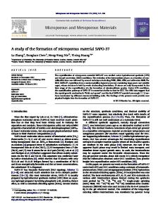
outcome—can be mapped onto firms’ profits. Furthermore, by allowing flexible strategic effects, we are able to capture both negative as well as positive effects of collocation. We also allow the strategic effects to be heterogeneous across firms. Finally, because our data is cross-sectional, the observed equilibrium outcome is the result of a steady-state, long-term equilibrium, where firms have made adjustments with regard to their choices (of entry). The complete information structure of the game fits this setting. We emphasize that we do not shy away from the complete information framework, despite the challenges of both multiple equilibria and heavy computational burden. Sections 3 and 4 discuss the methods we used to address these challenges. In addition to the discrete game, we jointly estimate a sales model that corrects the endogeneity problem with regard to firm entry, allowing us to evaluate the pure causal effect of a firm’s presence on mall sales. We supplement the market structure outcome with a sales model to jointly predict both the types of firms that will constitute a market and the total market sales, a crucially important factor to (mall) developers. We jointly utilize these two models to address the developer’s problem of where to create a market—that is, in our empirical setting, where to build a shopping mall. To address this problem, we adopt a Bayesian approach in which the posterior uncertainty of parameters properly factors into the location decision. We focus our attention to anchor stores because they are by definition the key tenants in a mall, occupying most of the mall’s gross leasable area (GLA) and generating much of the foot traffic (see Figure 1 for an example of a mall layout in terms of GLA). Anchor stores are competing department stores or retail chains; typical examples are Nordstrom, Macy’s, and Sears. We use data from the Directory of Major Malls, a data provider that supplies information about U.S. shopping centers and their tenants. We utilize information from 1,188 malls with 6,500 anchor stores to estimate our model.
There are several challenges involved in the joint modeling (and estimation) of market structure and market sales. First, as is the case with most discrete games, we face the problem of multiple equilibria, which makes it difficult to either define the likelihood for estimation or conduct accurate counterfactual policy simulations. As a result, past research has either scaled 3
back the problem (Bresnahan and Reiss, 1990; Berry, 1992), specified the sequence of moves (Berry, 1992; Mazzeo, 2002b), placed arbitrary assumptions related to equilibrium selection (Hartmann, 2010), or adopted a partial identification approach, i.e., estimated a range of parameters instead of point estimates (Ciliberto and Tamer, 2009). In this research, we address multiple equilibria by implementing the selection function method of Bajari, Hong, & Ryan (2010) to empirically estimate the equilibrium selection rule from the observed data. Second, to identify the pure causal effect of firm entry on total market sales, we must correct for the endogeneity issue—that is, do high expected market sales cause a firm to enter, or does firm entry cause high market sales? To address this problem, we include aggregate shocks both in our entry game and the sales model to isolate the pure causal effect of a specific firm’s entry on market sales. Finally, as is the case with the estimation of discrete games of complete information with multiple players, computational processing power is indispensable, especially in our setting, where we not only take into account equilibrium selection but also jointly estimate a model of market sales. We overcome this computational burden by utilizing general-purpose computing on graphics processing units (GPGPU), using multiple processing cores in a GPU of a graphics card to increase computation speed of our model estimation. The parallel computing of a GPU enables fast evaluation of simulated likelihood, a key step in our Bayesian estimation. It is worth discussing previous studies that connect entry decisions to other relevant variables concerning post-entry outcomes. Reiss and Spiller (1989) consider interactions between airlines' revenues and entry decisions, where the revenues are observed only when the airline enters and operates in the market. They propose a simple structure that allows for an analytic likelihood function to resolve this sample selection bias. Mazzeo (2002a) studies the effect of competition on the post-entry outcomes after correcting for the sample selection bias caused by firms' endogenous decisions to enter. Zhu, Singh & Manuszak (2009) analyze competition among Wal-Mart, Kmart and Target. They regress store revenues on market characteristics and presence of competing firms. The three chain stores' entry decisions are endogenous, which makes revenue data available only when they enter the market. The authors correct this bias by including correction terms for 4
endogenous market structure in the store-level revenue model. Ellickson and Misra (2012) propose a method that incorporates entry games and post-choice outcome data and corrects for sample selection biases. With an exception of Reiss and Spiller (1989), all the other papers adopt two-step estimation approaches which may be viewed as an extension of Heckman (1979). In the first step, entry game coefficients are estimated, and these estimates are corrected for selection biases in the second step. Two-step estimations are computationally less demanding than maximum likelihood estimation (MLE) which requires repetitive evaluations of the joint likelihood of entry games and post-entry equations. Despite the computational advantage, two-step estimation is known to perform poorly compared to an MLE. Please, see Nawata (1994) for details. We adopt the Bayesian approach that fully exploits the joint likelihood like an MLE. As mentioned earlier, we overcome the computational burden by using the GPGPU technology which computes the joint likelihood in parallel. Moreover, the speed advantage gained by GPGPU enables us to analyze nine players in our complete information entry games, compared to three players in Zhu, Singh and Manuszak (2009). Another difference between our setup and that of the aforementioned papers is that our endogeneity is not due to sample selection. We are interested in the mall's total revenues, not the individual department stores’ revenue. The total revenue data of the mall is available even if a particular department store does not enter the mall because the availability of revenue data is not related to the firm's decision. In terms of empirical context, our paper shares similarities with the work of Vitorino (2012), which also studies the entry behavior of anchor stores in a shopping mall. However, there are four key differences between her research and ours. First, she incorporates an incomplete information framework. Second, she uses the MPEC (mathematical problem with equilibrium constraints) method (Su and Judd, 2012) for estimation. Third, she does not explicitly address multiple equilibria. Finally, and most significantly, she focuses solely on market structure and does not examine the causal effect of firm entry on total mall sales. Our data, like hers, is cross-sectional, and thus the observed equilibrium outcome is the result of a steady-state long-term equilibrium, 5
which the complete information structure captures closer to reality than an incomplete information setting. In addition, while the MPEC method can estimate model parameters without directly addressing multiple equilibria, counterfactual analyses cannot be performed because there is no information about which equilibrium is selected. Conversely, we estimate the equilibrium selection function and consider all equilibria in both parameter estimation and counterfactual simulation analyses. Finally, we jointly analyze both mall configuration as well as mall sales to address the developer’s problem of where to construct a mall. Our results indicate that population and income are the key forces that drive retail stores’ profits: upscale retailers prefer to locate in affluent and populated areas, while midscale stores prefer to locate in lower-income and less-populated areas. We find that the negative effect of competition is prevalent within store categories, especially for discount and midscale stores, but positive agglomeration effects exist across store categories (discount and midscale). We also find substantial competitive effects not only within store categories but across store categories (midscale and upscale). Consistent with the results of a mall’s store configuration, population and income are also the main drivers of total mall sales. Furthermore, our results suggest that, above and beyond the effects of market characteristics, Dillard’s, Macy’s, and Nordstrom have a positive causal brand effect, whereas all discount stores have a negative causal brand effect on mall sales. Our counterfactual simulations reveal that certain stores would decide not to enter due to the competitive entry of other stores, even when market conditions are favorable. We find that a developer is moderately better off choosing a mall location that has high average income compared to large population. In terms of equilibrium selection, we find no evidence that the highest joint payoff equilibrium is more frequently selected, an assumption commonly used in the literature in both estimation and counterfactual policy simulations. The remainder of the paper is organized as follows. Section 2 discusses the data and industry details. In Sections 3 and 4, respectively, we present the model and estimation. discusses the estimation results and counterfactual analyses. Section 6 concludes.
2. Data and Industry Details 6
Section 5
Our mall configuration data comes from the Directory of Major Malls, a data provider that supplies information about shopping centers and their tenants operating in the U.S. Information is available on 7,411 malls operating as of December 2015 containing 264,868 stores, of which 27,431 are anchor stores. A typical shopping mall consists of a large cluster of retail stores sharing amenities such as restrooms, food courts, and customer parking facilities. Sometimes, logistical facilities such as loading docks and warehouses are also shared. General-purpose shopping centers are organized by size and trade area into the following categories: strip/convenience center, neighborhood center, community center, regional mall, and super-regional mall (see Table 1 for the definition of different types of shopping hubs by The International Council of Shopping Centers—ICSC, 2016).
According to the definition in Table 1, shopping hubs, generally referred to as shopping malls, are either regional or super-regional shopping malls. We define these malls as separate markets in which individual retail stores locate, a reasonable assumption because both regional and superregional malls are independent shopping hubs with space and capacity to provide a wide range of goods and services, operating in a large and separate geographical trade area. Therefore, we focus our analysis on regional and super-regional shopping malls and their tenant anchor stores. As previously mentioned, anchor stores are large chain stores, such as department stores or supermarkets, that drive the majority of customer traffic to a shopping mall. These retailers are typically classified into three broad categories—discount, midscale, or upscale—based on target customer segments (J.D. Power and Associates, 2007; Levy & Weitz, 2012). Focusing on price rather than service, discount department stores, such as Sears and Target, sell a variety of merchandise at a lower price than typical retail stores. Midscale department stores, including Macy’s and Dillard’s, offer a wide selection of both brand-name and non–brand name merchandise, seeking to offer good value to their customers. Upscale department stores sell goods at aboveaverage prices; their customers typically prefer exclusive designer brands and value customer service over low price. Examples include Nordstrom and Bloomingdale’s (see Table 2 for detailed categorization of each department store). 7
In addition to mall configuration, we obtain demographic data from the Scan/US demographic database, which includes population, size of household, and average household income within five miles of each shopping mall. Furthermore, we collect the location of each anchor store’s headquarters and compute the distance to every shopping mall in which it has a store. After data cleanup by excluding unusable observations that are missing information, we end up with 1,188 regional and super-regional shopping malls including 6,500 anchor stores for our empirical analysis. The summary statistics of the key variables are presented in Table 3.
A key reason that research on shopping centers is generally rare is the paucity of data; statistics on mall/store profitability such as rent and price are particularly difficult to obtain. The only available data is on market structure—that is, data on retail store configuration in a specific market (mall). To adequately investigate market formation and determinants of total market sales, one would need to supplement limited data with economic theory. Thus, a structural model of firm entry is suitable to address our research question.
3. Model We build a joint model of firm entry and sales to examine the formation of market structure and its effect on total market sales. First, we model the decision of a firm (anchor store) to enter a particular market (shopping mall) where a firm’s payoff depends on not only firm and market characteristics but also the entry decisions of other firms. Second, along with the model of entry decisions of firms, we jointly utilize a model of total market sales that corrects the endogeneity issue associated with firm entry—that is, do high expected market sales cause firm entry, or does firm entry cause high market sales? The previous literature on discrete games has focused on the configuration of market structure. We extend the market structure outcome with a sales model to jointly predict both the types of firms that would enter a specific market and total market sales, clearly important issues for mall developers. We jointly utilize these two models to address the developer’s problem of where to create a market—that is, where to build a shopping mall. 8
3.1. Discrete Game of Firm Entry We model the entry decisions of firms in a specific market as a simultaneous-move discrete game of complete information. Suppose there is a sequence of markets, indexed by m=1,…,M, where a market in our empirical context is defined as a retail shopping mall. In each market, there are J potential entrants (i.e., anchor stores), and the profit of firm j when entering market m is defined as J
pmj (am ) = pmj (amj = 1, am (- j ) ) = b j x mj + å djj'amj ' +j j xm + emj ,
(1)
j '¹ j
where am = (am 1 ,...amJ ) Î {0,1}J is the vector of action profiles of all firms in market m, with amj = 1 if firm j enters and amj = 0 otherwise. Similarly, am (- j ) is the vector of action profiles for all firms in market m other than firm j. The vector xmj represents the characteristics of firm j in market m, which may include market-level characteristics such as population, average income, and household size. The vector of parameters bj = (bj 1 ,..., bjK ) represents the marginal effect of firm and market-level characteristics on firm profit, and d j = (djj' )Jj '=1, j '¹ j represents the vector of strategic effects of other firms’ entries on firm j’s profit. Notice that we do not restrict these strategic effects to be negative but also allow them to be positive—that is, we allow negative competitive effects as well as positive agglomeration effects (Ciliberto and Tamer, 2009; Vitorino, 2012). The last two terms in Equation (1) are the unobserved components. The first term xm is the market-level shock common to all firms in a specific market, and the second term ejm is the firmmarket specific shock assumed to be independent across markets and firms. We assume that both terms follow a standard normal distribution and are observed by potential entrants but unobserved by the econometrician. It is important to recognize that the market-level shock common to all potential entrants in a market is the source of correlation among entrants’ payoffs. The market-level shock can be thought of as any factors that influence all firms in a market, such as highway access or the presence of other attractions (zoo, amusement park, etc.). We denote 9
j = (j1 ,..., jJ ) as the vector of marginal effects corresponding to market-level shocks—that is, the degree to which market-level shocks affect firm j’s payoff. We normalize the profit of a firm not entering the market to be zero.
3.2. Multiple Equilibria We assume that a pure strategy Nash equilibrium is observed in each market. Firm j enters market m if and only if pmj (amj = 1, am(-j ) ) > 0 . It is generally the case that a pure strategy Nash equilibrium is not unique in discrete games. Figure 2a and Figure 2b offer an illustrative example similar to that shown in Bresnahan and Reiss (1990). Suppose two firms, Nordstrom and Bloomingdale’s, are playing a simultaneous-move entry game of complete information. For simplicity, assume each player's payoff is dependent only on the strategic effect (entry choice) of the other player and an idiosyncratic shock. Thus, the profit function in Equation (1) has only the second and the last component. In such a case, the profits for Nordstrom in market m would be p mN = -dBN a mB + emN and the profits for Bloomingdale’s would be pmB = -dNB a mN + emB . If we
assume that entry is competitive ( d > 0 ), given a set of parameters, there would be a region in the (emN , emB) plane where one would observe more than one equilibrium outcome (shaded region in Figure 2a). Similarly, if the entry is complementary—that is, the profit function for Nordstrom is pmN = dBN a mB + emN and that of Bloomingdale’s is pmB = dNB a mN + emB ( d > 0 )— there would be a region in which an equilibrium outcome could either be all firms entering or none entering (shaded area in Figure 2b).
There are two potential problems associated with the multiplicity of equilibria. First, because there are specific regions (shaded regions in Figure 2a and Figure 2b) where no unique outcome exists, the model is termed incomplete (Tamer, 2003)—that is, we are not able to define the likelihood of certain types of outcomes. Second, counterfactual policy simulations cannot accurately predict an outcome, because we cannot determine which equilibrium is selected. To overcome this problem, researchers typically either simplified the scale of the problem, e.g., used 10
the number of firms rather than their identities (Bresnahan and Reiss, 1990), postulated a structure on the sequence of moves (Berry, 1992; Mazzeo, 2002b), set arbitrary assumptions with regard to equilibrium selection (Hartmann, 2010), or relied on a partial identification framework that estimated a range of parameters instead of point estimates (Ciliberto and Tamer, 2009). We mitigate the problem of multiple equilibria by empirically estimating—from the observed data— the selection rule proposed by Bjorn and Vuong (1984) and formalized by Bajari, Hong, & Ryan (2010).8 The detailed process is as follows. Let G be the set of pure strategy Nash equilibria given the discrete game payoffs. Thus, the probability that profile am is played is ì ï exp (kz (am )) ï ï if am Î G ìï1 if Y m (am ) = max Y m (am¢ ) ï ï ïï exp (kz (am¢ )) am¢ ÎG ï å ¢ ÎG a m r (am ; G) = í ï , where z a = m) ï í ( ï ïï ï ï ïï0 ï otherwise 0 otherwise ïî ï î
The joint payoff of firms taking action profile am is represented as Y m (am ) =
å
j
pmj (am ) and the
parameter k captures how often the highest joint payoff equilibrium is selected. For example, if k > 0 the highest joint payoff equilibrium is more likely to be selected instead of other equilibria. A discussion about the identification of k will be presented in the subsequent section. It is worth noting that the existing literature typically does not explicitly address equilibrium selection and makes arbitrary assumptions, such as that the highest total payoff equilibrium is always selected. As specified earlier, this research has two main objectives. First, we seek to provide projections about market structure—firm entry in the presence of other potential entrants—under particular market characteristics. Second, we utilize market structure information to predict market-level sales, informing developers about where to create a market. Performing such tasks require counterfactual analyses, that is, simulations of future discrete game outcomes 8
In our preliminary analysis, we tried another example of a selection rule in Bajari, Hong, & Ryan (2010). The estimation results were essentially identical.
11
where an equilibrium selection rule should be specified to choose equilibrium and predict the market structure.
3.3. Sales Model Along with a model to predict the market structure (type of firms in a specific market), to take into account the developer’s objectives, we consider the following model of total sales for a particular market as y m = lw m + s x xm + s n n m ,
(2)
where wm is the vector of characteristics of market m, such as population and average income. We also include a dummy variable for each anchor store (indicating its presence) in wm. Market-level unobservable effects are captured by xm and nm, both of which are assumed to come from the standard normal distribution. Furthermore, the two terms are assumed to be independent of each other as well as independent of market-store specific shocks emj in firm j’s profit function in Equation (1). As xm affects the entrant’s payoff, our model allows correlation between total sales of a market and its entrants’ profits, given all the observable variables. More specifically, the covariance between the error terms of an entrant firm j and the total sales of market m is
cov (jj xm + emj , sx xm + sn nm ) = jj sx . Next we consider the implication of the correlation between total market sales and entrants’ profits. Suppose there is a large market-level shock that affects both market sales and firms’ decisions to enter that market. Such shocks can be any unobservable (to the econometrician) elements not included in xmj and wm in equations (1) and (2), respectively. Thus, firm entry may be correlated with high sales because of the market-level shock, but not because an entrant draws more customers and boosts the total sales of the market. If the sales model in Equation (2) is run alone, the estimated effect of a firm’s entry will be biased because of the correlation between firm dummy variables and the regression error ( sx xm + sn nm ). Hence, we include the market-level
12
shock xm in both the entrant payoff in Equation (1) and the total market sales in Equation (2), and correct for the endogeneity bias by jointly estimating the parameters of the discrete game and the sales model.
4. Estimation We adopt a Bayesian approach because it provides a unified methodology for inference and decision. One of our ultimate goals is to propose a model that guides developers on where to build a shopping mall. Through the Bayesian approach, we can properly reflect the parameter uncertainty including the equilibrium selection when evaluating the desirability of each location choice. In addition, because we have more than 100 parameters in our empirical exercise, Bayesian inference on this large number of parameters turns out to be feasible. In this section, we discuss how we compute the posterior distribution for parameter inference. We use the Metropolis algorithm, one of the Markov Chain Monte Carlo (MCMC) methods that are common in Bayesian analysis when direct sampling from the posterior distribution is not feasible.
4.1. Likelihood Evaluation for Parameter Inference For parameter inference, we must compute the likelihood, the probability of observing the data given parameter values. Because the likelihood in our model does not have a closed-form solution, we use a frequency simulator similar to that of Ciliberto and Tamer (2009). We improve upon their simple simulator via methods we discuss in detail below. For notational simplicity, we will omit subscripts whenever the meanings are clear. Note that some components of w are whether anchor stores enter the mall (i.e., store dummies). Let w¢ denote all the variables except for the store dummies, such that w = (w ¢, a) . Variables in w¢ include population, average income, etc. The joint probability of observing firms’ entry decisions and market sales can be represented as
p (a, y | q, x, w ¢) = ò p (a | q, x, w ¢, x ) ⋅ p (y | a, q, x, w ¢, x ) f(x)d x 13
= ò p (a | q, x, x ) ⋅ p (y | a, q, w ¢, x ) f(x)dx ,
(3)
where f(.) is the density function of the standard normal distribution. The second equality holds because a is independent of w¢ conditional on (q , x ) , and y is independent of x given (a, q, w ¢) . We examine the two elements in Equation (3) separately. First, the marginal probability of observing firms’ entry decisions a Î {0,1}J in market m with common shock x is
p (a | q, x, x ) = ò r (a; G(e)) ⋅ f(e)de ,
(4)
where G(e) is the set of equilibria with explicit dependence on e. Because there is no closed-form solution for the set of equilibria G(e), to evaluate this we rely on a simple frequency simulator such as p (a | q, x , x ) »
1 R å r a; G(er ) , R r =1
(
)
(5)
where e 1 ,…,e R are J-dimensional independent standard normal draws. We refer to the simulator in Equation (5) the simple simulator. While the simple simulator can approximate the integral in Equation (4), it is not computationally efficient, because a majority of the draws may not provide any information to help determine the likelihood. Note that if one of the following holds for at least one j = 1,..., J :
(
)
(
)
i) ej < - bj x j + å j ¢¹ j djj¢a j + jj x and aj = 1 or ii) ej > - bj x j + å j ¢¹j djj¢a j + jj x and aj = 0 , then r (a; G(e)) = 0 because neither i) nor ii) is in equilibrium and thus not consistent with observation a. In other words, r (a; G(e)) = 0 represents the event that a firm enters when profits are negative or does not enter when profits are positive. Let E be the event in which either condition i) or ii) holds for some j=1,…,J. Then, a more efficient simulator can be written as
14
p (a | q, x , x )
( ) ò r (a; G(e)) ⋅ f(e | E )d e + Pr (E ) ò r (a; G(e)) ⋅ f(e | E )d e = Pr (E ) ò r (a; G(e)) ⋅ f(e | E )d e 1 » Pr (E ) å r (a; G(e )) R = Pr E c
c
c
c
R
c
r
r =1
where Ec is the complement of E and e 1 ,…,e R are drawn from the density f(e|E c ). Note that f(e|E c ) is the density of a truncated standard normal distribution. To draw e=(e 1 ,…,e R ), we draw each e j independently from a truncated standard normal, where the truncation level is set at
(
)
- bj x mj + å j ¢¹ j djj¢amj + jj xm and the truncation direction (left or right) is determined by amj.
( )
c The term Pr E is computed by the following product:
( )
Pr E c
J é æ öù = êêF ççç-b j x j - å djj¢a j ¢ - jj xm ÷÷÷úú ÷øú è j =1 êë ç j ¢¹ j û J
1-a j
J é ù æ ÷öú j ê1 - F çç-b j x j ÷ d a j x ¢ j j m å ÷÷ú j¢ ê çç è øúû j ¢¹ j êë
aj
where F(.) is the cumulative distribution function of the standard normal distribution. By avoiding simulation draws that give an obvious r (a; G(e)) = 0 , a significant advantage, our improved simulator performs more efficiently than the simple simulator in Equation (5). For example, assume that b j x j + å j ¢¹ j djj¢a j + j j x = 0 for all j=1,…,J with J = 9 —that is, the entry decisions of nine firms depend only on the draws of each e. In addition, assume that a=(1,…,1) is observed—that is, all firms enter. Thus, the event Ec is mapped onto the positive orthant of the J-dimensional Euclidean space of e. Via the simple simulator in Equation (5), a draw falls in E with probability 1 -
1 » 0.998 , and thus r (a; G(e)) = 0 . Hence, only 2 out of 1,000 draws on 29
average will lie in Ec and determine the value of the likelihood; whereas, in our improved simulator, all 1,000 draws will lie in Ec. Next, we discuss the computation of Γ(er), the set of all pure strategy Nash equilibria. To find all equilibria, we check whether each strategy profile is in equilibrium. For each market and each
15
draw of er, there are 2J strategy profiles to check for equilibrium. For example, if there are J = 9 potential entrants in 1,000 markets, and if we use 1,000 random draws of er for simulation, we would need to check 29 ´1,000´1,000=512 million cases for equilibria in each MCMC step, which would not be feasible using conventional computational methods. Because all these cases in a given MCMC step can be checked in parallel, we capitalize on the parallel-processing power of the GPGPU,9 a state-of-the-art technology that uses a graphics processing unit and its many cores to implement computation.10 The second part of the likelihood in Equation (3) is given by
p (y | a, q, w ¢, x ) =
1 æçy - lw - sx x ö÷ ÷÷ . fç sn çè sn ø÷
The details of our estimation procedure are laid out in the appendix.
4.2. Identification
We briefly discuss the intuition on what variation of the data helps make inferences on the parameters. For detailed arguments, see Bajari, Hong, & Ryan (2010). The idea is based on identification at infinity. We omit the market index m here. For each a-j, we can find large values of x such that playing a-j is a dominant strategy to all stores -j with probability close to 1. For these x values, small variation in xj identifies bj. Then, find x and x¢ such that bjx = bjx¢ and a-j differ only on aj’. The observed distribution of aj on x and x¢ identifies d. Given b and d, variation in j induces variation in correlation among firms’ payoffs and hence their entry decisions. Thus, when the equilibrium of the discrete game is unique, b, d and j are identified. 9
There are some papers that use graphics processing units to improve computation time. For example, Aldrich et al.
(2011) solve macroeconomic models, and Durham and Geweke (2014) propose a posterior simulator for Bayesian estimation. To the best of our knowledge, we are the first in the marketing literature to take advantage of the GPU technology. 10 Our implementation runs 500 times faster than a normal Matlab code. While our MCMC took approximately one day, a simple Matlab code without parallel processing would produce the same result in well over a year—that is, 500 days.
16
If equilibrium is not unique, the equilibrium selection plays a critical role in parameter estimation. Given values of the parameters (b, d, j), observations of markets with multiple equilibria will identify the selection probability r (am ; G) , in particular, k. Finally, the correlation between entry decisions am = (am1 ,...amJ ) and ym helps identify sx. The parameters l and sn are identified by variations in ym and wm. We have verified parameter identification numerically with datasets randomly generated according to our model. In the numerical exercise, a large number of observations make the posterior very close to the true parameter values.
5. Results
We first discuss the results of each firm’s profit function in Equation (1) and then discuss the results of the sales model in Equation (2). We follow by conducting several counterfactual policy simulations to address our research question of interest: where to construct a shopping mall.
5.1. Firm Profits Table 4 shows the parameter estimates with regard to market- and firm-specific effects and Table 5 shows estimates of the strategic spillover effects of the discrete game of firm entry; thus
combined, they represent the retail store’s profit function in Equation (1). There is clearly a substantial degree of heterogeneity via stores. We discuss in detail some noticeable patterns by store categories (discount, midscale, and upscale).
The constants are negative except for Macy’s and other midscale stores. This indicates that, given market characteristics, midscale stores are more likely to enter a specific market when not accounting for strategic effects of competitors’ entry.11
11
We will refrain from interpreting insignificant parameters.
17
The effect of population is positive for discount and upscale stores, indicating that these store types would prefer to locate in populated areas. In contrast, midscale stores would rather locate in less populated areas. The offerings of midscale stores typically consist of quality products similar to those at upscale stores, but with less service and at lower prices. Hence, midscale stores would find densely populated areas too costly (due to high labor and rental costs) to effectively operate in those areas. For upscale stores, such as Nordstrom and Bloomingdale’s, the inclination to enter populated areas is not surprising. Upscale stores, by definition, service upper-income segments of the population, which only exist in critical mass within highly populated areas. Correspondingly, parameters associated with average income (a proxy for purchasing power) indicate that Nordstrom and Bloomingdale’s prefer to locate in wealthy neighborhoods. On the other hand, the negative effect on average income implies that most discount and midscale stores prefer to locate in less affluent areas because they cater to low- to mid-income customers. The effect of household size is positive and significant for midscale stores, suggesting that large households with many family members appreciate the good value-per-price of midscale department stores. The effect of site size is positive for all midscale and upscale firms. Customers who shop in midscale and upscale firms value not only merchandise shopping but other amenities such as restaurants, cafes, movie theaters, valet parking, etc. Larger shopping malls have the space to provide more such amenities. The variable distance-to-HQ is insignificant for most firms, suggesting that there are no economic benefits by locating closer to a firm’s headquarters. All of our sample stores—anchor stores—are large chain department stores, which typically have achieved economies of scale in various dimensions and operate many distribution centers across the U.S. Hence, for most firms, distance to a firm’s headquarters does not seem to have a significant effect on the strategic choice of whether to operate in a particular market. Other market-level factors, such as population and purchasing power, seem to be more important when firms make strategic decisions to enter a specific market.
18
The market-level shocks represent any unobserved (by the econometrician) factors that influence firms in a particular market. Examples of such shocks include convenient transportation (highway access) and the presence (or proximity) of other attractions such as amusement parks. These common market-level shocks seem to have a strong influence on midscale but not so much for upscale department stores. The coefficient with regard to equilibrium selection is negative and statistically insignificant, providing no evidence that the highest joint payoff equilibrium is more frequently selected. This finding contradicts the previous literature that commonly assumed that the highest joint payoff equilibrium is chosen in both estimation and counterfactual policy simulations. In fact, our results actually show suggestive evidence (negative but insignificant parameter estimate with regard to equilibrium selection) that the highest joint payoff equilibrium is less commonly selected compared to other equilibria, implying stores do not seem to coordinate to achieve the highest joint payoff. The parameter estimates for the strategic effects of firm entry, shown in Table 5, are consistent with our earlier inference with regard to market- and firm-specific effects—for example, midscale stores’ reluctance to enter populated areas due to high operating costs. One can see that competition is the dominant effect within store categories, especially for midscale firms. Furthermore, midscale firms suffer from the entry of upscale firms, indicating competitive effects not only within store categories but across store categories. We would expect this result because product offerings at midscale firms are comparable to those at upscale firms but with less service at lower prices. In contrast, there is a positive agglomeration effect between discount and midscale firms. The product offerings of discount stores are typically different from those of midscale stores, and customers take advantage of one-stop shopping when these types of firms collocate. We will discuss these strategic effects in more detail when we perform our counterfactual policy simulations in Section 5.3.
5.2. Sales Model
19
Table 6 shows the results of the sales model in Equation (2). Consistent with the findings
from the discrete game of retail store entry, we find population and income are the key drivers of total mall sales. The main objective of Equation (2) is to infer the causal effect of each anchor store’s presence on total mall revenue. In order to precisely extrapolate the causal effect, we need to address the endogeneity issue associated with store entry. That is, do high expected sales cause a retail store to enter or does a store’s entry cause high mall sales? This question is especially critical for a developer who seeks to evaluate the causal effect of a specific department store’s presence on total mall sales.
As previously explained, we address the endogeneity issue through the common unobserved term xm in equations (1) and (2). Table 6 demonstrates that Dillard’s and Macy’s among midscale stores, and Nordstrom among upscale stores, have a positive causal effect on total mall sales. The positive causal effect can be due to two factors. First, the direct sales of a particular anchor store above and beyond the demand characteristics of the mall—that is, any effect on sales after controlling for market characteristics such as population and income. Second, the positive (or negative) spillover effect of an anchor store’s presence on total mall sales. Note that the spillover effect referred here is different from the strategic spillover effect in Equation (1). The former explains spillovers between anchor stores (competition and agglomeration) whereas the latter describes spillovers from a single anchor store to other smaller stores in a mall. Anchor stores attract mall customers through their brand and, as a result, draw smaller stores which increase total mall sales. We refer to the combination of these two effects as causal brand effects. Note that there is a negative causal effect for all discount stores. Because of harsh price competition, the presence of discount anchor stores discourages smaller stores from entering and, as a result, can have a diminishing effect on mall revenue. To illustrate the importance of our joint model (of firm entry and total market sales) that controls for the endogeneity of store entry, Table 7 shows the result of a sales model without common market-level shocks that affect store entry in a particular market—that is, without the
20
presence of common shock xm in equations (1) and (2). This result would be obtained by simply running an OLS (ordinary least square) regression of Equation (2). We can see there is a considerable difference between the results in Table 6 and Table 7. Although the directions of the parameter estimates are similar, most estimates become smaller in magnitude and statistically insignificant when the common shock is not included. For instance, consider the only significant firm-dummy variable, that of Nordstrom. The positive effect of Nordstrom’s entry is smaller than that in Table 6. Because any unobserved market-level shock that jointly affects firm entry and market sales, such as attractions or transportation convenience, can positively influence Nordstrom’s likelihood of entry, an OLS regression will underestimate the true causal effect of Nordstrom on total mall sales.
5.3. Counterfactual Analyses
Using the structural parameters estimated in the previous section, we examine the marginal effect of market characteristics on market structure and total market sales to guide the developer. For this analysis, first, we predict market structure—that is, compute the probability of each firm entering a market, given market characteristics—and then we compute the expected sales conditional on the configuration of market structure. For example, a developer needs to select a site to construct a new shopping mall. Choice of a site m is summarized as cm, where cm contains site characteristics (x and w¢) such as population and average income. The developer will choose the site that generates the highest total expected sales.12 Formally, let C be the set of choices. Then, the developer maximizes E[y | c] by choosing c ÎC such that
E éêëy | c ùúû = òò E éêëy | c, q, e, x ùúûdF(e, x)dp(q | data)
12
We assume that marginal cost is the same for all locations and that developer’s profits are proportional to total mall sales. Then, higher sales imply higher profits. With additional information on cost structures, it is easy to extend our analysis to more general cases.
21
where F(.) is the cumulative distribution function of an independent multivariate standard normal random vector and p(q|data) is the posterior distribution of the model parameters where data represents all data used in our model estimation. To compute the inner integral, given q, we simulate (er, xr) for r = 1,…,R. For each (er, xr), we compute the set of all pure strategy Nash equilibria G(er). If there exist multiple equilibria, entry decisions of potential entrants, ar, are
(
)
r drawn according to the equilibrium selection rule r a; G(e ; q) . This step is necessary to
determine w = (c, a ) because w includes firm dummy variables a. We use notation w(c,a) to denote w’s dependence on a as well as c. This procedure gives us the value of
E[y | c, q, e, x ] = lw(c, a r ) + sx x , where n in Equation (2) is ignored because its expectation is zero. Hence, we can compute the inner integral as 1
R
ò E éêëy | c, q, e, x ùúû dF(e, x) » R å lw(c, a
r
) + sx x r .
(6)
r =1
Finally, recall that we have samples of q, {q1,…, qS}, drawn from the posterior distribution, p(q|data) through our MCMC draws. Because each sample of q gives us one value of Equation (6), we can compute expected sales, given market characteristics c, as 1 E éêëy | c ùúû » S
S
S
R
å ò E éêëy | c, q, e, x ùúûdF(e, x) » SR å å lw (c, a ) + s x 1
s =1
r
x
r
.
s =1 r =1
Figure 3 shows the probability of selected firms entering conditional on different levels of
population. Consistent with the results of firms’ profit function in Table 4, we see that while the probability of entry for midscale stores, specifically Dillard’s and other midscale stores, decreases with
population,
the entry
probability
of upscale
stores,
specifically
Nordstrom
and
Bloomingdale’s, increases. However, contrary to Table 4, Macy’s entry probability actually increases with population. What explains this difference? We should note that a firm’s entry probability is a function of three components: the main effect from firm- and market-specific characteristics (Table 4), the within-category spillover effects (diagonal elements in Table 5), and the cross-category spillover effects (off-diagonal 22
elements in Table 5). As a result, even though Macy’s main effect with regard to population is negative, other midscale stores’ effect on population is also negative and thus discourages Macy’s competitors from entering the market. Less competition increases Macy’s likelihood of entry. Furthermore, discount stores are more likely to enter as population increases. Macy’s benefits from positive cross-category spillover effects, further increasing its probability of entry. Similarly, the entry decisions of Nordstrom and Bloomingdale’s depend on not only the main effect of population but also positive within-category spillover effects. We can see the amplifying effect reflected in the convex relation between population and the entry probability of Nordstrom and Bloomingdale’s shown in Figure 3.
To gain deeper insights into the spillover effects, consider the results of another analysis in which we examine the correlation between site size and firms’ probability of entry (Figure 4). Consistent with the main effects in Table 4, the entry probability of Target and other discount stores decreases as mall size increases. However, inconsistent with the (negative) main effects, Sears’ probability of entry seems to increase. Again, recall that our counterfactuals take into account not only the direct effect but also the equilibrium behavior of other firms and thus the spillover effect.
Let us examine the spillover effect more closely. Figure 5 separates the effect of site size on Sears’ profits into the direct (main) effect and the indirect (spillover) effect from other firms. The thick downward sloping dotted line represents the main effect of site size on Sears’ profits, and the thin lines represent the eight spillover effects from other firms—that is, the change in Sears’ profits due to the entry of other firms. The aggregate of all spillover effects is shown by the thick upward sloping dashed line. Finally, the sum of the main and overall spillover effects is represented by the thick solid line. Even though the main effect is negative, the overall effect of site size on Sears’ profits (and therefore the probability of entry) is positive, because the positive spillover effects are greater than the negative main effect.
23
Having explained all the working parts of our model, we are ready to return to our main research question: where to build a mall. Table 8 shows realistic scenarios facing a developer choosing a mall location. Site M possesses the average values of population and income as well as the average values of other variables in our data. The population of site A is 10 percent higher than that of site M (with the same average income as site M). Similarly, the average income of site B is 10 percent higher than that of site M (with the same population as site M). Other market characteristics in site A and B are set to the mean values in our data. We compare the effects of these changes in population and income in site A and B to determine which variable has a higher impact on mall sales.
Once again, because mall configuration outcome is a result of complex effects—main effect, within-category effect and cross-category effect—the final outcome may be different from the direction of the main effects in Table 4. For example, although the main effect of population is positive and highly significant for Target, the probability of Target’s entry actually falls as population increases (compare Target’s entry probability for site M and site A). This is due to the fact that in highly populated areas, the likelihood of entry increases for other discount stores, Target’s main competition. Because of the negative competitive effect, indicated by the diagonal elements in Table 5, Target’s profits (and thus the probability of entry) decreases with an increase in population. The results of mall configuration simulation suggests that more discount stores enter site A and more midscale and upscale stores enter site B, resulting in a higher number of anchor stores entering site B. Because of the greater number of stores along with the negative casual brand effect of discount stores (discouraging smaller stores from entering), site B (with higher income) outperforms site A (with larger population) by $14 million in total mall revenue.
6. Conclusion
In spite of the recent surge in e-commerce, brick-and-mortar retail, specifically in the form of large-scale shopping malls, is still the dominant venue for consumer purchases in the developed 24
world. Furthermore, coinciding with recent growth in real estate development in newly industrialized countries such as China, the construction of mass-scale shopping malls has experienced tremendous growth. Yet, there is little research about the dynamics governing the formation of the retail cluster—that is, what types of stores will join a shopping mall—and most importantly, the overall profitability of the mall. This paper develops a structural model of retail configuration with multiple equilibria and jointly estimates a discrete game of entry and total mall sales. Our analysis helps us assess (1) the types of stores that will join a shopping hub and (2) the expected financial performance of the shopping mall given its location and store configuration. We find population and income are the key drivers of retail stores’ profit; upscale stores locate in highly populated, affluent areas, whereas midscale stores locate in less populated, lower-income areas. Furthermore, both midscale and upscale stores prefer to locate in large shopping malls. Our analysis of strategic effects suggests the negative effect of competition is the dominant force within store categories, especially for discount and midscale stores, but positive agglomeration effects exist across store categories—discount and midscale. We also find substantial competitive effects not only within store categories but across store categories— midscale and upscale. We find that population and income are highly correlated with mall sales, and that Dillard’s, Macy’s, and Nordstrom have a positive causal brand effect, above and beyond the effects of market characteristics. Conversely, all discount stores have a negative causal brand effect on mall sales. Our counterfactual simulations suggest that some stores would decide not to join a mall despite favorable market conditions due to the expected competitive entry of other specific stores. Finally, we find that a developer is moderately better off choosing a mall location that has high average income compared to large population. Regarding equilibrium selection, we find no direct evidence that the highest joint payoff equilibrium is more frequently selected. In contrast, we find suggestive evidence that the highest joint payoff equilibrium is less commonly selected than other equilibria, challenging the common assumption used in the past economics and marketing literature.
25
Through our empirical application, we introduce three important methodological innovations. First, to the best of our knowledge, we provide one of the first empirical implementations of Bajari, Hong, & Ryan (2010) and consider all equilibria to estimate the equilibrium selection rule from the data. Second, we jointly estimate a discrete game of complete information with a sales model to identify the pure causal effect of a retail store’s entry on total mall sales. Finally, we utilize a state-of-the-art technology, GPGPU, using multiple processing cores of a graphics processing unit to significantly increase computational speed to consider and solve all equilibria, an effort that would not have been feasible with conventional computational methods. In summary, this research provides a rigorous yet practical framework to understand and evaluate why retail stores join a shopping mall and how their decisions affect mall revenue. Although our empirical application is in the retail shopping mall domain, our model can be extended and applied to a number of settings where a decision maker must choose among alternative sites to construct a market, for example, for transportation hubs such as airports or train stations. In addition, our modeling framework can be applied to assess the impact of regulatory factors on firms’ entry decisions and overall sales of site developers to gauge their implications on consumer welfare. We believe these substantive areas will be exciting venues for future research.
26
Appendix: Bayesian Estimation
This appendix provides the details of our Bayesian estimation procedure. To obtain the posterior distribution, we draw samples of q by the Metropolis algorithm. At each iteration t , the Metropolis algorithm draws q¢ from a proposal distribution, and determines if q¢ is accepted as a
{
}
posterior sample qt with probability max 1, p (q ') / p (qt-1 )
where p (q ) is the posterior
distribution of parameters. If q¢ is not accepted, we set qt = qt -1 . Recall p (q) = (prior density at q ) ⋅ (likelihood at q ) . Our choice of prior distribution for all parameters is set as the independent joint normal distribution with mean 0 and standard deviation 10. Because the likelihood does not admit a closed form, we rely on the simulated likelihood, explained in Section 4. Our choice of the proposal distribution is a random walk. The proposal distribution at iteration t is normal with mean vector qt and variance matrix s2V, where s is a positive number and V is a positive definite matrix. We tune the variance matrix to improve the performance of the Metropolis algorithm, a variation of Roberts & Rosenthal (2009) and Haario, Saksman, & Tamminen (2001). For s, we set our target acceptance probability between 0.1 and 0.3. If the number of accepted proposals in the last 100 iterations is below 10 or above 30, we adjust s accordingly. We set
(2.4)
2
V =
(dimension of q )
(covariance of t - 1 samples) + e (identity matrix)
at iteration t. Here, e is a very small positive number such that the second term guarantees positive definiteness of V. During the initial tuning stage, we run 100,000 Metropolis iterations. To evaluate the simulated likelihood, R=128 errors are generated once and the same errors are used throughout the entire Metropolis iterations. During the main MCMC stage, s and V are fixed. We set the matrix V equal to the one obtained from the initial tuning stage, and s is set to 0.6 which we determined by trial and error. For the main MCMC stage, R=1024 errors are simulated and fixed throughout the Metropolis 27
iterations. One million Metropolis iterations are run. Every 1000th samples are recorded and the first half of them is discarded as burn-in. Thus, we have 500 samples for parameter inference and counterfactual analyses. We have experimented with various numbers of iterations and sets of simulated errors, but the results were not qualitatively different. We run the estimation procedure with Matlab R2016b on 64 bit Windows 7, a desktop computer with Intel Core i7-6700K @4GHz, RAM 64GB, and a graphics card, GeForce GTX TITAN Black 6GB. The graphics card has 2880 CUDA (Compute Unified Device Architecture) cores which may be viewed as parallel processors. The graphics card executes our OpenCL kernel code to compute the simulated likelihood on these cores in parallel. The OpenCL kernel code execution is programmed to be controlled by our C++ code which is called by Matlab when evaluating the likelihood. As our dataset contains more than 1,000 shopping malls and R=1024 errors are simulated, an evaluation of the simulated likelihood requires solving for Nash equilibria of more than one million complete information entry games. All these games are solved in parallel by our graphics card. The main MCMC stage that evaluates the likelihood one million times took 20 hours.
28
References
Aldrich, E.M., Fernández-Villaverde, J., Gallant, A.R. & Rubio-Ramírez, J.F. (2011). Tapping the supercomputer under your desk: Solving dynamic equilibrium models with graphics processors. Journal of Economic Dynamics and Control, 35(3), 386-393. Bajari, P., Hong, H., & Ryan, S. P. (2010). Identification and estimation of a discrete game of complete information. Econometrica, 78(5), 1529-1568. Berry, S.T. (1992). Estimation of a model of entry in the airline industry. Econometrica, 60(4), 889-917. Bjorn, P.A., & Vuong, Q.H. (1984). Simultaneous equations models for dummy endogenous variables: a game theoretic formulation with an application to labor force participation. Working paper 537, California Institute of Technology. Bresnahan, T.F., & Reiss, P.C. (1990). Entry in monopoly markets. The Review of Economic Studies, 57(4), 531–553. Ciliberto, F., & Tamer, E. (2009). Market structure and multiple equilibria in airline markets. Econometrica, 77(6), 1791–1828. Durham, G., & Geweke, J. (2014). Adaptive sequential posterior simulators for massively parallel computing environments. Bayesian Model Comparison (Advances in Econometrics Vol. 34); Jeliazkov, I., Poirier, D.J., Eds, 1-44. Ellickson, P. B., & Misra, S. (2012). Enriching interactions: Incorporating outcome data into static discrete games. Quantitative Marketing and Economics, 10(1), 1-26. Haario, H., Saksman, E. & Tamminen, J. (2001). An adaptive Metropolis algorithm. Bernoulli, 7(2), 223-242. Hartmann, W.R. (2010). Demand estimation with social interactions and the implications for targeted marketing. Marketing Science, 29(4), 585–601. Heckman, J. J. (1979). Sample Selection Bias as a Specification Error, Econometrica, vol. 47 (1). 153-161. ICSC (The International Council of Shopping Centers) (2016). U.S. shopping-center classification and definitions. Accessed October 10, 2016, http://www.icsc.org/uploads/research/general/US_CENTER_CLASSIFICATION.pdf J.D. Power and Associates Reports (2007). Department Store Experience Study. Available at businesscenter.jdpower.com/news/pressrelease.aspx?ID=2007239. Levy, M., & Weitz, B.A. (2012). Retailing Management, 8th ed., McGraw-Hill Education. Mazzeo, M. J. (2002a). Competitive outcomes in product-differentiated oligopoly. Review of Economics and Statistics, 84(4), 716-728.
29
Mazzeo, M.J. (2002b). Product choice and oligopoly market structure. The RAND Journal of Economics, 33(2), 221–242. Nawata, K. (1994). Estimation of sample selection bias models by the maximum likelihood estimator and Heckman's two-step estimator. Economics Letters, 45(1), 33-40. Roberts, G.O. & Rosenthal, J.S. (2009). Examples of adaptive MCMC. Journal of Computational and Graphical Statistics, 18(2), 349-367. Su, C., & Judd, K. L. (2012). Constrained Optimization Approaches to Estimation of Structural Models. Econometrica, 80(5), 2213-2230. Tamer, E. (2003). Incomplete simultaneous discrete response model with multiple equilibria. Review of Economic Studies, 70(1), 147–165. Vitorino, M.A. (2012). Empirical entry games with complementarities: An application to the shopping center industry. Journal of Marketing Research, 49(2), 175-191. Zhu, T., Singh, V., & Manuszak, M. D. (2009). Market structure and competition in the retail discount industry. Journal of Marketing Research, 46(4), 453-466.
30
Table 1: U.S. Shopping Center Classification and Characteristics Type of Shopping Center Super-Regional Mall
Regional Mall
Community Center (“Large Neighborhood Center”)
Neighborhood Center
Concept
Similar in concept to regional malls, but offering more variety and assortment. General merchandise or fashion-oriented offerings. Typically, enclosed with inwardfacing stores connected by a common walkway. Parking surrounds the outside perimeter. General merchandise or convenienceoriented offerings. Wider range of apparel and other soft goods offerings than neighborhood centers. The center is usually configured in a straight line as a strip, or may be laid out in an L or U shape, depending on the site and design. Convenience oriented.
Average Size (Sq. Ft.)
Typical GLA* Range (Sq. Ft.)
Typical Number of Tenants
Trade Area Size
1,255,382
800,000+
NA
5-25 miles
589,659
400,000800,000
40-80 stores
5-15 miles
197,509
125,000400,000
15-40 stores
3-6 miles
71,827
30,000125,000
5-20 stores
3 miles
<30,000
NA
<1 mile
Attached row of stores or service outlets managed as a coherent retail entity, with on-site parking usually located in front of the stores. Open canopies may connect the store fronts, but a strip center does not have enclosed walkways linking the Strip/Convenience stores. A strip center may be configured 13,218 in a straight line, or have an “L” or “U” shape. A convenience center is among the smallest of the centers, whose tenants provide a narrow mix of goods and personal services to a very limited trade area. Source: The International Council of Shopping Centers, January 2017 * GLA: Gross leasable area
31
Table 2: Department Store Categorization Type
Definition
Stores
With a focus on price rather than service, discount department stores sell a variety of merchandise at a lower price than typical retail stores. Many Discount discount stores can be categorized as big-box stores, which offer a wide selection of products and grocery. Midscale department stores offer a wide selection of both brand-name Midscale and non–brand name merchandise, seeking to offer good value to their customers. Upscale department stores sell goods at above-average prices; their Upscale customers are more interested in exclusive designer brands and value customer service over low price. Source: J.D. Power and Associates (2007); Levy & Weitz (2011)
Kmart, Sears, Target, and Walmart
Dillard’s, JCPenney, Kohl’s, and Macy’s Bloomingdale’s, Neiman Marcus, Nordstrom, and Saks Fifth Avenue
Table 3: Variable Summary Statistics Variables Sears Target Other Discount Dillard’s Macy’s Other Midscale Nordstrom Bloomingdale’s Other Upscale Mall Sales ($) Population Age Household Size Household Income ($) Site Size (square feet) Open 2 (Malls opened during 1973 –1980) Open 3 (Malls opened after 1980) Sears Target Dillard’s Distance to Headquarter Macy’s (km) Nordstrom Bloomingdale’s
Note. Standard errors are reported in parentheses. Significance is in bold.
34
Table 8: Counterfactual Simulation—Where to Build a Mall? Site M
Site A
Site B
Population
380,914
419,005
380,914
Average Income
72,413
72,413
79,654
Sears
37.49%
36.29%
36.57%
Target
26.12%
26.07%
27.21%
Other discount
43.56%
43.99%
41.47%
Dillard's
23.45%
22.68%
20.14%
Macy's
42.12%
42.27%
44.33%
Other midscale
54.32%
52.95%
53.84%
Nordstrom
4.08%
4.60%
5.47%
Bloomingdale’s
0.08%
0.10%
0.12%
Other upscale
17.16%
16.63%
17.24%
1.89
1.93
2.07
Entry probability
Sales ($Billion)
Note: All variables are set to the mean values for site M. The population of site A is 10% higher than that of site M and the income of site B is 10% higher than that of site M. Other variables are set to their mean values for sites A and B.
35
Figure 1: Mall Floor Plan
South Coast Plaza, Costa Mesa, CA 92626, http://www.southcoastplaza.com/store-directory/
36
Figure 2: Multiple Equilibria—Illustrative Example a) Competitive Entry (Negative Spillover)
b) Complimentary Entry (Positive Spillover)
emB
emB
(1,1)
dNB (0,1) (1,0)
(0,1)
emN
emN
-dBN
dBN
(0,0) (1,1)
(0,0)
-dNB (1,0)
Profits of Nordstrom in market m are pmN = dBN amB + emN and those of Bloomingdale’s are pmB = dNBamN + emB (d > 0).
Profits of Nordstrom in market m are pmN = -dBN a mB + emN and those of Bloomingdale’s are pmB = -dNBamN + emB (d > 0).
37
Figure 3: Relation between Firm Entry and Population 1
Probability of Entry
0.8
0.6
0.4
0.2
0 -2
-1.6
-1.2
-0.8
-0.4
0
0.4
0.8
1.2
1.6
2
Population Dillards
Macys
Other midscale
Nordstrom
Bloomingdales
Note: Population is standardized value of log (population). That is, the x-axis represents standard deviations from the mean.
Figure 4: Relation between Firm Entry and Site Size
Probability of Entry
0.8
0.6
0.4
0.2
0 -2
-1.6
-1.2
-0.8
-0.4
0
0.4
0.8
1.2
1.6
2
Site Size
Sears
Target
Other discount
Note: Site size is standardized value of log (site size). That is, the x-axis represents standard deviations from the mean.
38
Figure 5: Main Effect vs. Spillover Effect of Site Size (Sears) 6 5 4
Payoffs
3 2 1 0 -1 -2 -2
-1.6
-1.2
-0.8
-0.4
0
0.4
0.8
1.2
1.6
2
Site Size Total
Direct
Spillovers
Target
Other discount
Dillards
Macys
Other midscale
Nordstrom
Bloomingdales
Other upscale
Note: The thick, downward sloping dotted line represents the main effect and the thick, upward sloping dashed line represents the aggregate spillover effect. The thick, upward sloping solid line is the sum of the main and the aggregate spillover effects. The eight thin lines are spillover effects from other firms. Site size is standardized value of log (site size). That is, the x-axis represents standard deviations from the mean.
Conference at Harvard Law School, Cambridge, Massachusetts, ... For more information on this or any other Aspen publication, please call 800-868-8437 or visit ...
major themes Mark emphasized. As you begin your study of Mark 4, jot down .... Our Amazing Bible Passport by Insight for Living Ministries softcover book.
It is one of the most developed city which will hold the World. University Games in 2011.So not only can you have a different life here, but also you can have a chance to attend the World University. Games ,meeting people from other countries. Page 2
In his recent article "Advent of Google means we must rethink our approach to education", Sugata Mitra argues that our education system needs to change. He suggests that the existence of modern technologies such as Google make the skills of the past
There was a problem previewing this document. Retrying... Download. Connect more apps... Try one of the apps below to open or edit this item. look where we ...
There was a problem previewing this document. Retrying... Download. Connect more apps... Try one of the apps below to open or edit this item. LYRICS Where We Meet.pdf. LYRICS Where We Meet.pdf. Open. Extract. Open with. Sign In. Main menu.
is where i'm dreaming of you. where your scent is a mist. and they look down at you. is where i want you to come with me. and everywhere else we will not meet. where doors are always locked. and longing makes you lonely. and waiting is your daily gri
Mar 29, 2013 - diffraction (PXRD). Scanning electron microscopy (SEM) was uti- lized to observe the morphological changes. Further, the nucleation and crystal growth were examined by atomic force microscopy. (AFM). The combination of these techniques
dedicated to the generation of new tissue using the principles of engineering in combination with an ... Address: PO Box: 71955-575, Shiraz 71955, Iran;. E-mail: ...
Shiraz NIOC Medical Education and Research Center, Shiraz, Iran. Biomaterials, as ... could be observed in publication of scientific articles on biomaterials too.
Over twenty colleges and universities in the US and UK have stopped doing business with the Coca-Cola company. Coca-Cola ... Contact us at: International ...
Mar 29, 2013 - For. DGC, SAPO-37 crystallizes from a semi-crysta lline layered precursor containing large pores and ... (DGC), was introduced years ago as an alternative method to HTS ... The silicon, aluminum, and phosphorous sources were fumed ...
Urgent Care. Center. You may need care quickly, but it is not an emergency, and your ... situations you can call your primary care physician at ... 24 Hour Health Information Program, help when you need it 24 hours a day/7 days a week.
suing a Denton Vacuum Desk II sputtering machine and observed using an .... [7] R. Jaeger, M.M. Bergshoef, C. Martin-I-Batlle, D. Schoenherr, G.J. Vancso,.
We build web businesses. Whoops! There was a problem loading this page. ... clients: http://flexi.ink/reviews. Whoops! There was a problem loading this page.
fire pit at the back of the church and have a grand ole time. September 6 ... direct your intentions for your, and the world's highest good. If you read this and .... the better it gets. All Is Well. STONE OF THE MONTH. MOONSTONE. Has healing affinit
There was a problem previewing this document. Retrying... Download. Connect more apps... Try one of the apps below to open or edit this item. Read Write ...