1

A Distributed Algorithm to Achieve Transparent Coexistence for a Secondary Multi-hop MIMO Network Xu Yuan, Member, IEEE, Xiaoqi Qin, Student Member, IEEE, Feng Tian, Member, IEEE, Yi Shi, Senior Member, IEEE, Y. Thomas Hou, Fellow, IEEE, Wenjing Lou, Fellow, IEEE, Scott F. Midkiff, Senior Member, IEEE, and Sastry Kompella, Senior Member, IEEE

Abstract—The transparent coexistence (TC) paradigm allows simultaneous activation of the secondary users with the primary users as long as their interference to the primary users can be properly canceled. This paradigm has the potential to offer much more efficient spectrum sharing than traditional interweave paradigm. In this paper, we design a distributed algorithm to achieve this paradigm for a secondary multi-hop network. For interference cancelation (IC), we employ MIMO at secondary nodes. We present a distributed iterative algorithm to maximize each secondary session’s throughput while meeting all IC requirements under TC. By maintaining two local sets for each node, we can keep track of the node’s IC responsibility. Although no explicit node ordering is maintained in our distributed algorithm, we prove that our distributed data structure at each node (with the use of two local sets) can be mapped to an explicit global node ordering for IC among all nodes in the network. This guarantees that each active node’s degree-of-freedoms (DoFs) allocated for IC is feasible at the physical (PHY) layer. Our algorithm is iterative in nature and all steps can be accomplished based on local information exchange among the neighboring nodes. We present simulation results to show that the performance of our distributed algorithm is highly competitive when compared to an upper bound solution from the corresponding centralized problem. Index Terms—Primary network, secondary network, spectrum sharing, coexistence, distributed algorithm, multi-hop network, MIMO, interference cancelation.

I. I NTRODUCTION A spectrum sharing paradigm is defined by how the secondary and the primary users achieve coexistence. In [3], Goldsmith et al. outlined three main paradigms, namely interweave, underlay, and overlay. Interweave is a simple but conservative approach that follows the traditional interference avoidance paradigm. Under interweave, a secondary network is allowed to access radio spectrum only when it is not in Manuscript received July 9, 2015; revised January 18, 2016; accepted May 27, 2016. An abridged version of this paper was presented at IEEE IPCCC, Austin, TX, USA, 2014 [21]. The associate editor coordinating the review of this paper and approving it for publication was W. Wang. X. Yuan, X. Qin, Y.T. Hou, W. Lou, and S.F. Midkiff are with the Virginia Polytechnic Institute and State University, Blacksburg, VA 24061, USA. (email: {xuy10, xiaoqi, thou, wjlou, midkiff}@vt.edu). F. Tian is with the Nanjing University of Posts and Telecommunications, Nanjing, Jiangsu 210003, China. (e-mail:[email protected]). Y. Shi is with the Intelligent Automation Inc., Rockville, MD, 20855, USA. (e-mail: [email protected]). S. Kompella is with the U.S. Naval Research Laboratory, Washington, DC 20375, USA. (email: [email protected]).

conflict with the primary users in time, frequency, or space [2], [5], [17]. On the other hand, overlay is considered an aggressive spectrum sharing paradigm as it encourages proactive cooperation between the primary and secondary networks in data forwarding [7], [8], [11], [15], [23], [26]. In terms of spectrum sharing efficiency and network performance, overlay represents the ultimate coexistence paradigm, although its actual adaptation and deployment may still be years away due to the need of significant change in primary users’ behavior. In this research, we focus on the underlay paradigm, which is considered as a major step forward beyond the interweave paradigm while requiring minimal change on the primary network. The underlay refers to that secondary users may be active simultaneously with the primary users in the same vicinity and in the same frequency, as long as the secondary user’s interference to primary users are negligible (or below a given threshold). Underlay coexistence paradigm has been explored in [1], [10], [24], [25]. In [1], Gao et al. studied the transmission strategies for a MIMO secondary link with a primary link. They proposed a secondary transmission strategy consisting of environment learning, channel training, and data transmission. In [24], Zhang and Liang studied the transmission strategy for a single secondary MIMO link coexisting with multiple primary receivers with interference-power constraints. In [25], Zhang et al. studied the secondary-link beamforming pattern to achieve the coexistence of a single secondary link with multiple primary links. They aimed to maximize the secondary user’s throughput while keeping the interference temperature at the primary receivers below a certain threshold. In [10], Kim and Giannakis studied the coexistence of multiple secondary links with one primary link. They proposed a distributed resource allocation algorithm to maximize the weighted sum rate of secondary links under a transmit power constraint at the secondary transmitters and an interference power constraint at the primary receiver. All these prior efforts were from information theoretic perspective. A common limitation of these prior efforts is that they are all limited to very simple network settings, e.g., several nodes or link pairs, all for singlehop communications. In a recent study [19], we explored the underlay paradigm for a secondary multi-hop network under the name of transparent coexistence (TC). Under TC, there is no change on the primary network’s behavior. It uses the spectrum as it wishes

2

and is not concerned with the needs of the secondary network. On the other hand, the secondary network is allowed to access the spectrum in the same time, frequency, and location with the primary network, as long as its activities are “invisible” to the primary network. Such transparency is achieved by having the secondary network proactively cancel its interference to the primary network with powerful physical (PHY) layer techniques so that the primary nodes do not feel the presence of the secondary nodes. As a result, simultaneous activation of the secondary network along with the primary network is possible. In [19], we developed centralized mathematical models to characterize (i) inter-network interference cancelation (IC) relationships between two networks – secondary transmitters need to cancel their interference to the primary receivers while secondary receivers need to cancel the interference from the primary transmitters; and (ii) intra-network IC – secondary nodes need to perform IC within their own network so that data can be transported successfully within the secondary network. The results in [19] showed the concept of achieving TC for a multi-hop primary and secondary network through a centralized solution. But it is also desirable to have a distributed solution to achieve TC. The main contribution of this paper is the development of a distributed scheduling algorithm for the secondary network to achieve TC with the primary network, while maximizing its own network throughput. For IC, we assume each secondary node is equipped with MIMO, while there is no requirement on the primary nodes. We employ a MIMO IC model that was developed in [14] to keep track of degree-of-freedoms (DoFs) allocation for transporting data streams (i.e., spatial multiplexing (SM)) and IC. It was shown in [14] that this IC model is efficient in DoF allocation while guaranteeing feasibility in the final solution. By feasibility, we mean there exists a feasible precoding and decoding vector for each data stream at the PHY layer. However, this model is centralized in nature and requires to maintain a global node ordering among the secondary nodes in the network, which is not possible in a distributed network environment. In this paper, instead of maintaining a global node ordering, we only maintain two local sets at each node to keep track of the node’s IC responsibilities. We show how to establish, maintain, and update these two local sets at each node in each iteration of our distributed algorithm. Our distributed algorithm increases the data stream on each active link iteratively based on local computation. Since the nodes in the two local sets of a node directly affect the node’s IC responsibility, our algorithm attempts to switch nodes in the two sets if it can improve the IC structure. Although no explicit node ordering is maintained in our distributed algorithm, we prove that our distributed data structure at each node (with the use of two local sets) can be mapped to an explicit global node ordering for IC among all nodes in the network. From this global node ordering for IC among all nodes, we show there exist a set of feasible precoding vectors at each secondary transmitter and a feasible set of decoding vectors at each secondary receiver so that all data (in both primary and secondary networks) can be transported free of interference. Through numerical results, we show that the iterative distributed algorithm that we propose offers competitive performance when compared with an upper

TABLE I N OTATION P T F˜ L˜

The The The The

S S Ai F L

The The The The The

Primary Network set of nodes in the primary network number of time slot in a frame set of sessions in the primary network set of active primary links Secondary Network set of nodes in the secondary network number of secondary nodes in the network, S = |S| number of antennas at secondary node i ∈ S set of sessions in the secondary network set of secondary links

bound result from centralized optimization. The remainder of this paper is organized as follows. In Section II, we describe our problem. Section III presents the design of an iterative distributed algorithm to achieve TC for a secondary multi-hop network. In Section IV, we present a feasibility proof of our distributed algorithm at the PHY layer. In Section V, we analyze the complexity and overhead of our distributed algorithm. Section VI presents numerical results and demonstrates the competitive performance of the proposed distributed algorithm. Section VII concludes this paper. II. P ROBLEM D ESCRIPTION In this paper, we consider a multi-hop primary network (with a set of nodes P) and a multi-hop secondary network (with a set of nodes S) that are co-located in the same geographical area, as shown in Fig. 1. Table I lists the notation in this paper. The primary network is assigned a certain spectrum band for its communication. Suppose scheduling is done in the time domain, with T time slots in a frame. For the primary network, it performs scheduling for transmission/reception without any consideration of the secondary network. A secondary node, however, is allowed to transmit in a time slot only if it is able to cancel its interference to its neighboring primary receivers. We assume the primary nodes are single antenna nodes. Suppose that there is a set of sessions F˜ in the primary network P. Each session has a source node and a destination node and traverses multihop relay nodes as needed. The route from a session’s source node to its destination node is given a prior, which may be found by some standard routing protocols (e.g., AODV [12], DSR [9]). Denote L˜ as a set of links in the network that ˜ Suppose the set are traversed by the active sessions in F. of links L˜ is operating under a feasible scheduling solution ˜ where (for transmisson/reception) for the primary sessions F, interference at a primary receive node is avoided either through time slot or sufficient spatial separation. Since each primary node has only a single antenna, it can transmit at most one data stream to another node in a time slot. For the secondary network, we assume each node is equipped with MIMO, which offers IC capability that is needed to achieve TC. We assume the number of antennas at a secondary node i ∈ S is Ai . For the secondary network S, suppose that there is a set of sessions F in S. Similar to a primary session, a secondary session has a source node, a destination node, and traverses multi-hop relay nodes as

3

S1

P1

Primary nodes

Secondary nodes

Fig. 1. A multi-hop secondary network co-located in the same area as a multi-hop primary network.

needed. The route from a secondary session’s source node to its destination node is again given a priori. Denote L as the set of links that are traversed by any session in F. We use DoFs at a secondary node (no more than the number of antennas at the node) to represent its available resources. A DoF can be used for SM or IC. For SM, transmitting one data stream requires one DoF at the transmitter and one DoF at the receiver. In practice, the data rate carried in each data stream may vary with different channel conditions. For simplicity, we assume that the fixed modulation and coding scheme (MCS) is used for a link’s data stream transmission, and one data stream in one time slot corresponds to one unit data rate. On the other hand, DoF consumption for IC depends on whether the IC is done at the transmitter or receiver. We use a simple example to illustrate this point. In Fig. 2, suppose P1 and P2 are a pair of primary transmit and receive nodes, while S1 and S2 , S3 and S4 are two pairs of secondary transmit and receive nodes. Suppose that both the primary nodes P1 and P2 have one antenna, and the secondary nodes S1 , S2 , S3 , and S4 are each equipped with 4 antennas (4 DoFs). P1 is transmitting 1 data stream to P2 , S1 is transmitting 1 data stream to S2 , and S3 is transmitting 2 data stream to S4 . For the interference from S1 to S4 , either transmitter S1 or receiver S4 can cancel this interference. If S1 is to cancel this interference, then it will use 2 DoFs since S4 is receiving 2 data streams; if S4 is to cancel this interference, then it will use 1 DoF since S1 is transmitting 1 data stream. Note the difference in DoF consumptions in IC by different nodes. As described, to achieve TC, the secondary nodes have the sole responsibility to cancel interference to/from the primary nodes (i.e., inter-network interference) and interference within the secondary network (i.e., intra-network interference). In this example, for inter-network IC, secondary nodes S2 and S4 need to cancel the interference from primary transmit node P1 with 1 DoF, respectively; the secondary transmit nodes S1 and S3 need to cancel their interference to primary receive node P2 with 1 DoF, respectively. For intra-network IC, the interference from S1 to S4 needs to be cancelled, either by S1 (with 2 DoF) or by S4 (with 1 DoF) as discussed earlier; the interference from S3 to S2 needs to be cancelled, either by S3 (with 1 DoF) or by S2 (with 2 DoFs). To successfully perform inter- and intra-network IC, it is

S3

1

1

2

S2

P2

S4

Fig. 2. A simple example illustrating SM and IC. A solid line represents the primary link, a dashed line represents a secondary link, and a dotted line represents an interference.

crucial for the secondary nodes to have accurate channel state information (CSI). We propose one particular scheme for the secondary nodes to obtain CSI between themselves and their neighboring primary and secondary nodes while remaining transparent to the primary nodes. The main idea of the scheme is to have the primary and secondary nodes send out known pilot signal so that neighboring secondary nodes can estimate CSI. This is the practice for current cellular networks and we will employ such a mechanism for both the primary and secondary networks. Suppose the pilot sequences from the primary and secondary nodes are publicly available (as in cellular networks). After the primary and secondary nodes send out the pilot sequences, the neighboring secondary nodes can compare the known pilot sequences with the actual received sequences signal from the senders for channel estimation. Based on the reciprocity property of a wireless channel, the estimated CSI can also be used as CSIT (channel state information at transmitter side) when the secondary node becomes a transmit node. Therefore, each secondary node can obtain complete CSI between itself and a neighboring primary or secondary node. There are many other schemes that have been proposed to address this issue (see, e.g., [4], [13], [18], [19], [21], [27]). We omit their discussions here to conserve space. But the point here is that there exist schemes that we can use to obtain the necessary CSI for the secondary nodes to perform inter- and intra-network IC. In our design of distributed algorithm for the secondary nodes to achieve TC, we consider a throughput maximization problem, with the objective of maximizing the minimum achievable session rate (in terms of data streams) among all secondary sessions. We choose this objective since it focuses on the worst case (minimum) achievable secondary session throughput, which ensures fairness across all secondary sessions. III. A D ISTRIBUTED A LGORITHM We propose a distributed scheduling algorithm to the throughput maximization problem while meeting all IC requirements for the secondary nodes. As described in our network setting, the set of sessions F˜ in the primary network are transmitting under a given feasible scheduling solution. To have the secondary sessions operate in the same set of time

4

TABLE II S TATE INFORMATION AT EACH

i

Symbol si (t) Bi (t) Yi (t) λSM i (t) λIC i (t)

Fig. 3. Maintaining two local sets at node i to distinguish IC responsibility between node i and its neighboring nodes.

λRM (t) i α ˜ i (t) β˜i (t)

slots (to achieve TC), we employ MIMO at the secondary nodes for IC. The algorithm that we propose is an iterative greedy algorithm. We consider one link (from the set of links L) at a time and try to increase the data streams on this link by 1 in this iteration. This increment is successful only if the transmitter, receiver and neighboring nodes of this link have enough remaining DoFs to cancel this new interference on neighboring primary and secondary nodes. As discussed earlier, an interference can be canceled either by a secondary transmit or receive node. For efficient and feasible IC, a global node ordering scheme proposed in [14] would be useful. But such a global node ordering scheme is centralized in nature. Nevertheless, it gives us some hints in our design of distributed algorithm. We propose to maintain two local sets at each node to keep track of the IC responsibility between this node and neighboring nodes. For example, at each secondary node i ∈ S, we maintain one local set Bi (t) to store i’s neighboring nodes that require node i to use its DoFs for IC and the other local set Yi (t) to store i’s neighboring nodes that use their own DoFs for canceling interference to/from node i (see Fig. 3). Note that there is no explicit node ordering among the nodes in sets Bi (t) and Yi (t). By maintaining these two sets (with Bi (t) before node i and Yi (t) after node i), we have achieved the desired efficiency in IC locally at node i. We will discuss the feasibility issue in Section IV. The use of two local sets Bi (t) and Yi (t) at each secondary node i is centerpiece in our design of distributed scheduling algorithm to achieve TC. In our algorithm, we will exploit these two sets at each node to its fullest extent to achieve IC at the secondary nodes while meeting the resource constraints (limited DoFs at each node). In particular, when we find that a data stream cannot be further increased on a bottleneck link, we will consider moving some nodes from one local set into the other set so that the DoFs at a node can be reallocated. This step is called adjusting IC responsibility in our algorithm (Step 3) and is a critical component to maximize the performance of our algorithm. At any iteration when this IC responsibility adjustment is not successful (and thus the number of data streams on the associated link cannot be further increased) for all time slots in a frame, our algorithm terminates.

αi (t) βi (t) zi,j (t)

NODE

i

Definition The status of node i in time slot t. si (t) = Tx, Rx or Idle. The set of nodes that node i allocates DoFs for IC to/from them in time slot t. The set of nodes that allocate their own DoFs for IC to/from node i in time slot t. The number of DoFs that node i has allocated for SM in time slot t. The number of DoFs that node i has allocated for IC in time slot t. The number of remaining DoFs at node i ∈ S in time slot t, IC i.e., λRM (t) = Ai − λSM i i (t) − λi (t). The total number of data streams from node i’s neighboring primary transmitters in time slot t. The total number of data streams received by node i’s neighboring primary receivers in time slot t. The total number of data streams from node i’s neighboring secondary transmitters in time slot t. The total number of data stream received by node i’s neighboring secondary receivers in time slot t. The number of data streams from transmit node i to receive node j.

A. State Information at Secondary Nodes The state information that needs to be maintained at a secondary node (say i) is shown in Table II. Local sets Bi (t) and Yi (t): For each interference involving node i, it can be canceled by either node i or the other node involved in this interference. To explicitly distinguish who is responsible for IC for each interference, we maintain two local sets Bi (t) and Yi (t) at each node i, as shown in Figure 3. We denote Bi (t) as the set of secondary nodes that node i (i ∈ S) allocates DoFs to cancel interference to/from them, and denote Yi (t) as the set of secondary nodes that allocate their DoFs to cancel interference to/from i. At the beginning of our algorithm, we initialize Bi (t) and Yi (t) as empty sets, i.e., Bi (t) = ∅ and Yi (t) = ∅ for i ∈ S. Accounting of DoF resource: In Table II, zi,j (t) represents the number of data stream transmitted from node i to node j. IC λSM i (t) and λi (t) represents the number of DoFs allocated for SM and IC at secondary node i in time slot t, respectively. λRM (t) represents the number of remaining DoFs at a node i i in time slot t. At the beginning of our algorithm, the status of each node i ∈ S is set to Idle, i.e., si (t) =Idle for t = 1, 2, · · · , T . Then, the initial DoF allocation for SM IC and IC at each node is 0. We have λSM i (t) = λi (t) = 0, RM λi (t) = Ai and zi,j (t) = 0 for i, j ∈ S, t = 1, 2, · · · , T in the initialization stage. α ˜ i (t) and β˜i (t) are constants and are calculated based on active sessions in the primary network. These can be derived by the secondary nodes through monitoring/sensing of the neighboring primary nodes’s activities. On the other hand, the initial values for αi (t) and βi (t) are 0. For these state information, except that α ˜ i (t) and β˜i (t) are IC constants, the values for si (t), Bi (t), Yi (t), λSM i (t), λi (t), RM λi (t), zi,j (t), αi (t) and βi (t) are variables and will be updated during each iteration of the algorithm. B. Step 1: Choosing a Link To make a rate increment of each session by 1 DoF is equivalent to increasing the DoF on each active link by 1 DoF

5

•

Fig. 4.

Four cases of link status.

if each active link is traversed by 1 session. In the general case when an active link is traversed by multiple sessions, we need to increase the DoFs on this active link by multiple times, each for one session. In our distributed algorithm, we choose an active link for increment during an iteration. If a link is traversed by multiple sessions, then it is necessary to represent the link multiple times so that each session traversing this link is to be considered for data stream increment. Suppose there are k sessions traversing a link l ∈ L. Then we represent link l by k logical links. We want to set a round robin for these logical links for rate increment so that each logical link is considered once in each cycle. To do this, we employ the so-called distributed ranking algorithm by Zaks [28]. This algorithm was designed to solve the problem of sorting and ranking n processors in a distributed system. The input is an initial value unique for each processor. The output is a ranking of all n processors. To apply the distributed ranking algorithm, we assign an initial value for each logical link. Each initial value is generated randomly and guaranteed to be unique (under a reasonably good random number generator). We let the transmitter of each logical link to maintain the logical link’s rank. After a logical link obtains its rank, it will know precisely when it will be considered for data stream increment. C. Step 2: Data Stream Increment After we identify a logical link (in Step 1), our algorithm will try to increase one data stream on the selected link, while satisfying IC constraints and transparency to the primary network.1 We first present the necessary conditions under which one more data stream can be added on the link in a time slot. Then we describe how to update state information on the nodes that are involved in this increment. Sufficient Conditions for Data Stream Increment. We now discuss when the number of data streams on a chosen link can be increased by 1 in a given time slot. Suppose link (i, j) is the link. Then both nodes i and j first check their current status (“Tx”, “Rx”, or “Idle”). Some cases can be clearly ruled out for consideration, i.e., si (t) = Rx or sj (t) = Tx. In these cases, link (i, j) cannot be considered for data stream increment in time slot t and we move to the next time slot (t + 1) immediately. When link (i, j) is suitable for data stream increment, there are four possible statuses as shown in Figure 4. The sufficient conditions for data stream increment on link (i, j) are as follows. Case (a): si (t) = Idle and sj (t) = Idle.

•

si (t) = Idle: Since node i is idle, the local sets Bi (t) and Yi (t) are empty. We need to establish the sets Bi (t) and Yi (t) (see Figure 3) to decide the IC relationships between node i and its neighboring secondary receive nodes that will be interfered by i. We can put all these neighboring receive nodes in time slot t either in Bi (t) or Yi (t). – If all neighboring receive nodes are put into Yi (t), then the interference from node i to them will be canceled by these receive nodes. The following two conditions must be satisfied: (i) the total number of DoFs at node i should be greater than the total number of data streams received by its neighboring primary receivers, i.e., Ai > β˜i (t), (ii) all secondary receivers that are in Yi (t) must have at least one remaining DoFs to cancel one more data stream interference from node i. – If all neighboring receive nodes are put into Bi (t), node i needs to cancel its interference to all these neighboring receive nodes. The following condition must be satisfied: the total number of DoFs at node i is more than the sum of data streams received by both neighboring primary and secondary receivers, i.e., Ai > β˜i (t) + βi (t). sj (t) = Idle: Similar to node i, we put node j’s neighboring transmit nodes in either Bj (t) or Yj (t). The sufficient conditions for j are similar as i, we omit its discussion here.

If the conditions for si (t) = Idle and sj (t) = Idle are both satisfied, we proceed with this increment and update state information at nodes i, j and their neighboring nodes according to Figure 5 and Figure 6. State update at idle node i and neighboring receiver k 1. If si (t) = Idle: 2. Update si (t) = Tx; λSM (t) ← λSM (t) + 1; i i RM λRM (t) ← λ (t) − 1; zi,j (t) ← zi,j (t) + 1. i i 3. If Yi (t) ← {Neighboring active secondary receivers.} RM ˜ 4. Update λIC (t) ← λRM (t) − λIC i (t) ← βi (t); λi i i (t); 5. For each receive node k ∈ Yi (t): IC 6. Bk (t) ← Bk (t) ∪ {i}; λIC k (t) ← λk (t) + 1; λRM (t) ← λRM (t) − 1. k k 7. Else if Bi (t) ← {Neighboring active secondary receivers.} RM ˜ 8. Update λIC (t) ← λRM (t) − λIC i (t) ← βi (t) + βi (t); λi i i (t). 9. For each node k ∈ Bi (t): Yk (t) = Yk (t) ∪ {i}.

Fig. 5.

Pseudocode to update state information when si (t) = Idle.

State update at idle node j and neighboring transmitter k 1. If sj (t) = Idle: SM 2. Update sj (t) = Rx; λSM j (t) ← λj (t) + 1; λRM (t) ← λRM (t) − 1; zi,j (t) ← zi,j (t) + 1. j j 3. If Yj (t) ← {Neighboring active secondary transmitters.} 4. Update λIC ˜ j (t); λRM (t) ← λRM (t) − λIC j (t) ← α j j j (t) 5. For each transmit node k ∈ Yj (t): IC 6. Bk (t) ← Bk (t) ∪ {j}; λIC k (t) = λk (t) + 1; λRM (t) = λRM (t) − 1. k k 7. Else if Bj (t) ← {Neighboring active secondary transmitters.} 8. Update λIC ˜ j (t) + αj (t); λRM (t) ← λRM (t) − λIC j (t) ← α j j j (t). 9. For each k ∈ Bj (t): Yk (t) ← Yk (t) ∪ {j}.

Fig. 6.

Pseudocode to update state information when sj (t) = Idle.

1 We

drop the fine distinction between “link” and “logical link” when there is no confusion.

Case (b): si (t) = Tx and sj (t) = Idle.

6

si (t) = Tx : In this case, the following conditions must be satisfied if node i wants to increase one more data stream on link (i, j): (i) node i has at least one remaining DoF for SM, i.e., λRM (t) ≥ 1; (ii) each receive node i k ∈ Yi (t) has at least one remaining DoF to cancel the new interference from node i. • sj (t) = Idle : This case has been discussed in Case (a). If the conditions for si (t) = Tx and sj (t) = Idle are both satisfied, we proceed with this increment and update state information at nodes i, j and their neighboring nodes according to Figure 6 and Figure 7. •

State update at transmit node i and neighboring receiver k 1. If si (t) = Tx: 2. Update λSM (t) ← λSM (t) + 1; λRM (t) ← λRM (t) − 1; i i i i zi,j (t) = zi,j (t) + 1. 3. For each receive node k ∈ Yi (t): IC RM 4. Update λIC (t) ← λRM (t) − 1. k (t) ← λk (t) + 1; λk k

Fig. 7.

Pseudocode to update state information when si (t) = Tx.

Case (c): si (t) = Idle and sj (t) = Rx. • si (t) = Idle: This case has been discussed in Case (a). • sj (t) = Rx: In this case, the following condition must be satisfied if node j wants to increase one more data stream on link (i, j): (i) node j has at least one remaining DoF for SM, i.e., λRM j (t) ≥ 1; (ii) each transmit node k ∈ Yj (t) has at least one remaining DoF to cancel its interference to node j. If the conditions for si (t) = Idle and sj (t) = Rx are both satisfied, we proceed with this increment and update state information at nodes i, j and their neighboring nodes according to Figure 5 and Figure 8. State update at receive node j and neighboring transmitter k 1. If sj (t) = Rx: SM RM 2. Update λSM (t) ← λRM (t) − 1; j (t) ← λj (t) + 1; λj j zi,j (t) = zi,j (t) + 1. 3. For each transmit node k ∈ Yj (t): IC RM 4. Update λIC (t) ← λRM (t) − 1. k (t) ← λk (t) + 1; λk k

Fig. 8.

Pseudocode to update state information when sj (t) = Rx.

Case (d): si (t) = Tx and sj (t) = Rx. The case for si (t) = Tx has been discussed in Case (b) and sj (t) = Rx has been discussed in Case (c). If the conditions for si (t) = Tx and sj (t) = Rx are both satisfied, we proceed with this increment and update state information at nodes i, j and their neighboring nodes according to Figure 7 and Figure 8. Recall that there are T time slots in a time frame. Node activities (both primary and secondary) and interference patterns in each time slot are different. If the data stream increment operation described above fails in the first time slot, we try it again in the second time slot and so forth, until a data stream increment is successful in a time slot or fails after all T time slots. D. Step 3: Adjusting a Node’s IC Responsibility If the sufficient conditions at either node i or node j cannot be satisfied, we move on to this step. The only reason why link (i, j) fails to increase one data stream in step 2 is the lack of DoF resources at some nodes (bottleneck nodes), i.e.,

node i, j or nodes in Yi (t) and Yj (t). Since a node’s local sets B and Y directly affects its DoF consumption for IC, we will try to swap some nodes between the sets B and Y, and thus change their IC responsibilities. For example, if node k is short on DoFs, we can move some node m ∈ Bk (t) to Yk (t), thereby transferring the IC responsibility from k to m. Through this change, some new DoF resources for the bottleneck node k become available, possibly allowing a new data stream increment to be made on the link under consideration. The main idea of this step is as follows. For each time slot t, we identify the set of bottleneck nodes (denoted as D(i,j) (t)), which do not have enough remaining DoF resources should one more data stream is added onto link (i, j). For each node k ∈ D(i,j) (t), we adjust node k’s IC responsibility by moving some other nodes in Bk (t) to Yk (t). To ensure feasibility, only a subset of nodes (denoted as B¯k (t)), B¯k (t) ⊆ Bk (t), is eligible for moving from Bk (t) to Yk (t). After identifying B¯k (t) for k, we consider nodes in B¯k (t) in the order of nonincreasing remaining DoFs, i.e., starting with the one that has the maximum remaining DoF (denoted as node a) if it is moved to Yk (t). If this movement is infeasible, then our attempted adjustment fails in this time slot and we move on to the next time slot. Otherwise, we move a from Bk (t) to Yk (t) and update their state information. After this movement, if a new data stream can be added on link (i, j), we are done. Otherwise, we continue moving the next node in B¯k (t) that has the maximum remaining DoF (denoted as node b) to Yk (t) following the same process. This step terminates upon a new data stream can be successfully added on link (i, j) or all nodes in D(i,j) (t) are considered for all time slots in a frame. In the rest of this section, we give more details for this idea. Finding bottleneck nodes D(i,j) (t): D(i,j) (t) can be easily found by identifying those nodes that would need more DoFs than their remaining DoFs should one more data stream were added on link (i, j). Node sequence in D(i,j) (t): To consider nodes one at a time in D(i,j) (t) in a distributed environment, we could use a token to pass along from one node to the next so that at any time, only one node is considered for adjustment. There is no preference on which node to start but for the rest of the discussion, we assume that we start with node i, then j, before the other nodes in D(i,j) (t). Note that a token is passed to the next node in D(i,j) (t) only if the adjustment in the previous node is successful. Otherwise, the algorithm moves on to the next time slot in the frame. Finding eligible subset nodes for swapping: Suppose the token is now passed onto node k ∈ D(i,j) (t). To adjust node k’s IC responsibility, we want to move one or more nodes in Bk (t) to Yk (t), thus relieving node k’s IC responsibility for these nodes. But for feasibility, not every node in Bk (t) is eligible for swapping. Now we discuss how to identify a subset of nodes B¯k (t) that are eligible to be moved to Yk (t). By “eligible”, we mean that when we move the subset of nodes from Bk (t) to Yk (t), the IC responsibilities for all other nodes in B¯k (t) and Yk (t) are not affected. We propose a sufficient condition to check whether or not a node is an eligible node as follows.

7

... y x

a

x

send est requ

...

(a) An illustration of determining the eligibility of receive node a ∈ Bk (t).

...

...

... a

m

(b) Steps involved in determining the eligibility of receive node a ∈ Bk (t).

Fig. 9. Determining the eligibility of receive node a ∈ Bk (t) when node k is a transmit node.

Suppose node k is a transmitter. Then it can consider those receive nodes in Bk (t) for moving to Yk (t). We denote c ← b as node b cancels interference to or from c. For a receive node a ∈ Bk (t), it can be moved to Yk (t) if the following conditions are satisfied. For each transmit node x ∈ Ya (t) that needs to do IC to a (i.e., a ← x), there cannot exist a receive node y ∈ Yx (t) that y handles IC from x (i.e., x ← y), and k handles IC to y (i.e., y ← k) (see Figure 9 (a)). That is, there does not exist a receive node y, such that the following IC relationship holds: a ← x ← y ← k. If this condition is satisfied and a’s remaining DoFs is at least one after moving to Yk (t), a is an eligible node; otherwise, a is not. In Section IV, we will show that this condition can guarantee IC feasibility among all nodes. To do this check, we have node a send a request for state information to those transmit nodes in Ya (t). Upon receiving this request, each transmit node x ∈ Ya (t) will send its state information Yx (t) to node a (see Figure 9(b)). Upon receiving this state information, node a can check whether some receive nodes in Yx (t) are also in Bk (t). If none of these receive nodes are in Bk (t) and a’s remaining DoFs is at least one after moving to Yk (t), then a is eligible. Otherwise, a is not eligible. The above discussion is for the case when node k is a transmit node. The case when node k is a receive or idle node can be handled in a similar manner. Moving node(s) in B¯k (t) to Yk (t): Assume node a ∈ B¯k (t) has the maximum remaining DoFs after moving to Yk (t). If B¯k (t) = ∅, there is no eligible node and we move to next time slot immediately. Otherwise, at node k, we move a from B¯k (t) to Yk (t) while at node a, we move k from Ya (t) to Ba (t), and update their state information as follows. • Case sk (t) = Tx or sk (t) = Rx: In this case, k only needs to release one DoF. Since at node k, we move a from Bk (t) to Yk (t) while at node a, we move k from Ya (t) to Ba (t), then at least one DoF can be released from k. The node k updates the state information based on Figure 10, and the node a updates its state information based on Figure 11. • Case sk (t) = Idle: Recall that for the bottleneck node

k in D(i,j) (t), it might be i, j, or node in Yi (t) or in Yj (t). Since Yi (t) represents the set of i’s neighboring receive nodes that should allocate DoFs to cancel interference from node i, and Yj (t) represents the set of j’s neighboring transmit nodes that should allocate DoFs to cancel their interference to node j, then all nodes in Yi (t) and Yj (t) are active nodes. Therefore, node k can only represent node i or node j. Let’s consider the case when node k is node i. The case when node k is node j is similar. Recall that when sk (t) = Idle, both Bk (t) and Yk (t) are empty. We establish Bk (t) and Yk (t) by putting all neighboring active nodes in either Bk (t) or Yk (t). Clearly, putting all neighboring receive nodes in Yk (t) will add additional IC burden on all these nodes in Yk (t) and may require adjusting each node’s IC responsibility in Yk (t). On the other hand, putting all neighboring receive nodes to Bk (t) will not have this issue as the IC responsibility on those nodes in Bk (t) are not affected and we only need to focus on adjusting node k’s responsibility with one node in Bk (t). We adopt the latter approach and put all neighboring receive nodes in Bk (t) and set Yk (t) = ∅ (see Figure 12 (a)). For each node p ∈ Bk (t), node k is added to Yp (t). ∑sn (t)=Rx SM ˜ Therefore, λIC k (t) = n∈Bk (t) λn (t) + βk (t), where β˜k (t) is the total number of data streams received by node i’s neighboring primary receivers, and λRM k (t) = Ak − λIC (t). We start to put node a (the node in B¯k (t) k that has the maximum remaining DoFs after movement) (see Figure 12 (b)) into Yk (t) . Both nodes k and a’s state information is updated based on Figures 10 and 11, respectively. For the new sets, if a new data stream can be added on link (i, j), we are done. Otherwise, we continue to move another node b ∈ B¯k (t) that has the maximum remaining DoFs after movement following the same process (see Figure 12(c)). The process terminates if node k has at least one remaining DoF or B¯k (t) = ∅. For the latter case, the adjustment fails and we move on to the next time slot.

IV. F EASIBILITY In our design of distributed algorithm, for each node k, we put its neighboring nodes in two sets: Bk (t) and Yk (t). For the set of nodes in Bk (t), node k is responsible to cancel its interference to them if k is a transmit node or cancel the interference from them if k is a receive node. For the ease of understanding, we can consider the set of nodes in Bk (t) being positioned before node k while the set of nodes in Yk (t) being positioned after node k. That is, there is a relative ordering among nodes in Bk (t), node k, and nodes in Yk (t). Under this notion, node k, being positioned after the set of nodes in Bk (t), is responsible to cancel interference to/from nodes in Bk (t). Note that we did not make a finer distinction of the relative positions (or ordering) among the set of nodes in Bk (t) or Yk (t). In this section, we show that the coarse set-based ordering Bk (t) or Yk (t) at node k locally can in fact be mapped into a

8

State Information Update at node k 1. Update Bk (t) ← Bk (t) − {a}, Yk (t) ← Yk (t) ∪ {a}; 2. If sk (t) = Tx: IC SM 3. Update λIC k (t) ← λk (t) − (λa (t) − zk,a (t)); RM (t) + (λSM (t) − z λRM (t) ← λ k,a (t)); a k k 4. Else if sk (t) = Rx: IC SM 5. Update λIC k (t) ← λk (t) − (λa (t) − za,k (t)); RM (t) + (λSM (t) − z λRM (t) ← λ a,k (t)); a k k 6. Else if sk (t) = Idle: IC SM RM RM SM λIC k (t) ← λk (t) − λa (t); λk (t) ← λk (t) + λa (t); Fig. 10.

State Information Update at node a 1. Update Ya (t) ← Ya (t) − {k}, Ba (t) ← Ba (t) ∪ {k}; 2. If sk (t) = Tx: IC SM 3. Update λIC a (t) ← λa (t) + (λk (t) − zk,a (t)); RM (t) − (λSM (t) − z λRM (t) ← λ (t)); k,a a a k 4. Else if sk (t) = Rx: IC SM 5. Update λIC a (t) ← λa (t) + (λk (t) − za,k (t)); RM (t) − (λSM (t) − z λRM (t) ← λ a,k (t)); a a k 6. Else if sk (t) = Idle: No Changes; Fig. 11.

Update state information at k.

Update state information at a.

a b

b k

a

...

...

...

k

k

a b

...

...

...

Fig. 12.

(a) Before movement

(b) Move a to Yk (t)

(c) Move b to Yk (t)

An illustration of movement process when node k is an idle node.

“global node ordering” for IC among all the nodes explicitly. More formally, we give the following definition. Definition 1: A global node ordering for IC is a list of nodes where the position of a node in the list determines its IC responsibility. Based on this list, a node is responsible for canceling interference to/from these nodes that are before itself in the list; a node does not need to cancel the interference to/from those nodes that are after itself in the list as that interference will be canceled by those nodes. Based on this definition, we show if there exists a global node ordering for IC among the active nodes in the network, then there exists a set of feasible precoding vectors at each secondary transmitter and decoding vectors at each secondary receiver so that all data (in both primary and secondary networks) can be transported free of interference using zeroforcing technique on the secondary nodes. That is, if a global node ordering for IC exists among the active nodes, then there exist feasible precoding and decoding vectors at the PHY layer to implement the desired IC and SM in the network. Lemma 1: Upon the termination of the distributed algorithm, there exists a global node ordering for IC among all nodes in each time slot t. Proof: Before we start our algorithm, all secondary nodes are inactive and there does not exist any ordering among the nodes. Since none of the primary nodes perform IC (due to the fact that potential interference among the primary nodes is handled by interference avoidance through time slot), we can envision a list containing all active primary nodes with arbitrary order among them. We will build upon this list to establish a global node ordering for IC. To achieve TC, all interferences to/from primary network is canceled by the secondary nodes. Following the definition of global node ordering for IC, the secondary nodes must be placed after the primary nodes. We now show that we can

maintain a global node ordering for IC at each iteration. Upon termination of the last iteration, the list remains a global node ordering for IC. If a link fails to increase one data stream at the end of any iteration, the current global ordering for IC will not be affected. So in our proof, we only need to discuss the case that we can increase one data stream upon the end of the an iteration. Our proof is based on induction. For the first iteration, a secondary link is selected for data stream increment. We append the secondary transmit and receive nodes of this link at the end of the current list. Since there is no IC relationship between the secondary transmit and receive nodes of the chosen link, we can put transmit node either before or after the receive node. The new global ordering list consists of all active primary nodes, plus the secondary transmit and receive nodes of the chosen link. Since we can increase one data stream on this link, all interference from this link’s transmit node to the neighboring primary receivers can be canceled by this transmit node, and all interference from neighboring primary transmitters to the chosen link’s receive node can be canceled by this receive node. Obviously, this new list satisfies global node ordering for IC by definition. Upon the end of n-th iteration, suppose there exists a global node ordering for IC. Then, we show that at the end of the (n + 1)-th iteration, there still exists a global node ordering for IC. Denote link (i, j) as the link chosen for data stream increment during the (n + 1) iteration. We consider two cases: (i) a data stream can be added onto (i, j) without adjusting node ordering; (ii) a data stream can be added onto (i, j) but requiring adjusting node ordering: • (i) We first consider that one data stream can be added onto (i, j) without adjusting node ordering in the current global node ordering list. We take node i as an example. There are two cases:

9

– Node i is not yet on the current global node ordering list. In this case, si (t) =Idle and our algorithm will put node i’s neighboring receive nodes (not including j) either in Bi (t) or Yi (t). Since all these neighboring receive nodes are active, they already have their positions in the current global ordering list in a previous iteration. If node i’s neighboring receive nodes are put in Bi (t), it is the same as putting node i after these neighboring receive nodes. If node i’s neighboring receive nodes are put in Yi (t), it is the same as putting node i before these neighboring receive nodes. In either case, other nodes’ relative ordering on the current global node ordering list is not affected, and thus IC responsibilities among them remain the same. Since one data stream can be added onto link (i, j) successfully, node i must be able to cancel interference to these nodes in Bi (t) (if these receive nodes are put into Bi (t)), or the interference from i can be canceled by these nodes in Yi (t) (if these receive nodes are put into Yi (t)). Therefore, on the new list, each node is responsible for canceling interference to/from these nodes that are before itself in the list; each node does not need to cancel the interference to/from those nodes that are after itself in the list as that interference will be canceled by those nodes. By definition, the new list satisfies the global node ordering for IC. – Node i is already on the global node ordering list. In this case, si (t)=Tx and the node i only performs data stream increment. There is no new node to be added to the list or none of the nodes change its position in the list. Therefore, the current ordering list is the same as that in the n-th iteration and satisfies the global node ordering for IC.

•

The case for node j is similar and we omit its discussion here to conserve space. (ii) We then consider that one data stream can be added onto (i, j) but requiring adjusting node ordering in the current global node ordering. We assume that node k ∈ D(i,j) (t) is under consideration for adjustment. Suppose k is a transmit node. Recall that a necessary condition for a receive node a ∈ Bk (t) to be moved to Yk (t) is that: for each transmit node x ∈ Ya (t) that needs to do IC to a (i.e., a ← x), there cannot exist a receive node y ∈ Yx (t) that y handles IC from x (i.e., x ← y), and k handles IC to y (i.e., y ← k) (see Figure 9(a)). That is, there does not exist a transmit node x and a receive node y, such that the following IC relationship holds: a ← x ← y ← k. Therefore, when node a is chosen to move from Bk (t) to Yk (t), node a’s IC responsibility for other transmit nodes, and node k’s IC responsibility for other receive nodes will not change, except changing the position of k and a (i.e., moving a after k). Since this change is successful, a is able to cancel the interference from k and other transmit nodes that are before k. Therefore, the new list satisfies the global node ordering for IC. The discussion when k is a receiver is similar.

pm

p1 ...

...

...

pM ...

r1 Primary node

...

...

...

...

rn

rN

... i

Secondary node

Fig. 13. A secondary transmit node i performs IC to neighboring primary and secondary receive nodes in a time slot t.

Therefore, we conclude that after the (n + 1)-th iteration, the new list satisfies the global node ordering for IC. Based on the above discussion, we conclude that upon the termination of the distributed algorithm, we have a global node ordering for IC. Theorem 1: There exists a set of feasible precoding vectors at each secondary transmitter and a feasible set of decoding vectors at each secondary receiver so that all data (in both primary and secondary networks) can be transported free of interference based on the global node ordering for IC. Proof: We first consider a secondary transmit node i on the global node ordering list, as shown in Figure 13. The dashed arrows represent the interference from node i to those receive nodes that are before node i on the global node ordering list. The nodes p1 · · · pM are i’s neighboring primary receivers, while nodes r1 · · · rN are i’s neighboring secondary receivers. Suppose that i transmits z(i,j) data streams to secondary node j. Denote uqi as an Ai × 1 transmit weight vector at i for each data stream q (1 ≤ q ≤ z(i,j) ), and vjq as an Aj × 1 receive weight vector at receiver node j to receive data stream q. Since each primary link only transmits one data stream, we use u1p and vp1 to denote the primary node p’s (p ∈ {p1 , · · · , pM }) transmit and receive vectors . Denote H(i,b) (b ∈ {p1 , · · · , pM , r1 , · · · , rN }) as the Ai × Ab channel gain matrix between nodes i and b. We assume a rich scattering environment, where all channels Hi,b have full rank and independent with each other. To successfully transmit z(i,j) data stream from node i to its intended receive node j, the transmit node i should cancel all its interference to primary receive nodes p1 to pM and secondary receive nodes r1 to rN . Then, we should have the following constraints: (uqi )T H(i,j) vjq = 1 , (uqi )T H(i,j) vjd (uqi )T H(i,pm ) vp1m

(1 ≤ q ≤ z(i,j) ) ,

(1)

=0,

(1 ≤ q, d ≤ z(i,j) , d ̸= q) , (2)

=0,

(1 ≤ q ≤ z(i,j) , 1 ≤ m ≤ M ) , (3)

(uqi )T H(i,rn ) vrdn = 0 ,

(1 ≤ q ≤ z(i,j) , 1 ≤ n ≤ N, 1 ≤ d ≤ z(sn ,rn ) ) ,

(4)

where sn is the transmit node which transports z(sn ,rn ) data streams to secondary receive node rn . The number of constraints from (1) and (2) are (z(i,j) )2 . ∑M The number of constraints from (3) is z(i,j) m=1 1. The ∑N number of constraints from (4) is z(i,j) n=1 z(sn ,rn ) . The ∑M total number of constraints is therefore (z(i,j) m=1 1 + ∑ N (z(i,j) )2 + z(i,j) n=1 z(sn ,rn ) ). Recall that in our algorithm, in either step 2 or step 3, the total number of DoF consumption

10

cannot be more∑than the total number of ∑ DoFs at a node. M N We have, z(i,j) m=1 1 + (z(i,j) )2 + z(i,j) n=1 z(sn ,rn ) ≤ ∑M ∑N z(i,j) ( m=1 1 + z(i,j) + n=1 z(sn ,rn ) ) ≤ z(i,j) Ai . That is, the total number of constraints is no more than z(i,j) Ai . Since the precoding vector uqi is an Ai × 1 vector for each data stream q (1 ≤ q ≤ z(i,j) ), the total number of variables at the transmit node i is z(i,j) Ai and the number of variables is no less than the number of constraints. On the other hand, since the channels H(i,b) are full rank and independent with each other, it can be shown that the constraints in (1), (2), (3), and (4) are linearly independent with each other based on [14]. So for any given vjq (1 ≤ q ≤ z(i,j) ), we are guaranteed to construct feasible precoding vectors uqi (1 ≤ q ≤ z(i,j) ) at transmit node i. The proof that we can construct the feasible decoding vectors vjq (1 ≤ q ≤ z(i,j) ) at the secondary receive node j (for any given precoding vectors uqi (1 ≤ q ≤ z(i,j) )) is similar to the transmit node i. We omit its discussion here to conserve space. Based on the above discussions, there exist feasible precoding/decoding vectors at the secondary nodes. Therefore, there exists a set of feasible precoding vectors at each secondary transmitter and a feasible set of decoding vectors at each secondary receiver so that all data (in both primary and secondary networks) can be transported free of interference. This completes the proof. V. C OMPLEXITY AND OVERHEAD A NALYSIS A. Complexity Analysis We now show that the overall computation complexity of the distributed algorithm is polynomial time. Step 1 (ranking of active secondary links) is done only once. As shown in [28], this step can be done in O(S 2 ). The iteration of our algorithm involves steps 2 and 3. We now analyze the complexity of each iteration and the number of iterations required in the algorithm. In step 2, nodes i and j (for a chosen link (i, j)) need to check the feasibility of increasing one more data stream over at most T time slots. The worst case scenario is that both nodes i and j are idle (case (a) in Fig. 4). Since both nodes i and j need to check the number of remaining DoFs of each of their neighboring nodes and the number of DoFs used for SM by these nodes, the complexity of this operation is O(2S). Afterward, nodes i and j, and their neighbors, need to update their DoF allocation status. The complexity of this operation is O(S). Since there is a total of T time slots, the total complexity of this step is T · O(2S + S) = O(ST ). In step 3, nodes i and j, as well as their neighboring nodes attempt to adjust IC responsibility in at most T time slots. During each time slot, the computation consists of three parts: (i) identifying the subset of nodes D(i,j) (t), which has a complexity O(S); (ii) identifying the set of nodes B¯k (t) for each k ∈ D(i,j) (t), which has a complexity of O(S 2 ). Since the number of nodes in D(i,j) (t) is at most S, the total complexity for (ii) is O(S ∗ S 2 ) = O(S 3 ); (iii) adjusting the IC responsibility for each node k ∈ D(i,j) (t), and updating each node’s state information, which has a complexity O(S).

Since there is a total of T time slots, the total complexity of step 3 is T · O(S + S 3 + S) = O(T S 3 ). Since each node has A antennas and there are L active links in the network, the number of iterations of our algorithm is at most O(LA). Therefore the overall complexity is O(S 2 + O(LA) · [O(ST ) + O(T S 3 )]) = O(LAT S 3 ). B. Overhead Analysis In a distributed environment, the success of this distributed algorithm relies on the message exchanges in the common control channel among the secondary nodes. Since it is hard to quantify overhead precisely induced by this algorithm, we develop an upper bound for the total volume of message exchanges among the secondary nodes in this algorithm. In what follows, we analyze the volume of message exchanges in each step. In Step 1, message exchange is required to sort the links in the network. Here, we employ the distributed ranking algorithm based on the results in [28], which require O(S 2 ) message exchanges in the worst case. As for Step 2 and Step 3, there are at most O(T LA) iterations. To find the volume of message exchange in each iteration, we analyze each step separately. In Step 2, both nodes i and j need to communicate with their neighboring nodes to check the remaining number of DoFs and the number of DoFs for SM by these nodes. This requires O(S) message exchanges in each time slot. Afterward, nodes i and j need to send messages to their neighboring nodes to update their DoF allocation status. This requires O(S) messages. So the total volume of message exchange in Step 2 is O(S). In Step 3, for each bottleneck node, the volume of message exchange with a node in Bk (t) is O(2) and there are at most O(S) nodes in Bk (t). So Step 3 requires O(S) message exchanges for each bottleneck node. Since there are at most S bottleneck nodes, the total volume of message exchanges induced by Step 3 is O(S 2 ). Putting things together, the total volume of message exchange induced by Step 2 and Step 3 is O(T LA(S + S 2 )) = O(T LAS 2 ). By adding the message exchanges in the three steps together, this distributed algorithm requires O(S 2 + T LAS 2 ) message exchanges in the worse case. VI. S IMULATION R ESULTS In this section, we present simulation results to demonstrate the performance of the proposed distributed algorithm. We compare our results with the centralized methods as discussed in [21]. Since the centralized problem formulation is MILP, which is NP-hard in general, we cannot obtain the optimal solution for comparison. Instead, we will compare the performance of our algorithm to an upper bound of the objective for the centralized problem. Such an upper bound can be obtained by running CPLEX for a given termination time. Clearly, such a comparison approach is very aggressive and conservation. This is because the optimal objective value (not obtainable) to the centralized problem lies between the upper bound and the feasible solution obtained by our distributed algorithm. Therefore, if the feasible solution from our distributed algorithm is somehow close to the upper bound by CPLEX, then we can

11

claim that our solution (objective) is even closer to the optimal objective and thus is competitive. A. Simulation Setting We consider a secondary CR network co-locates with a primary network within a 100 × 100 area. For generality, we normalize the units for distance, bandwidth, and data rate with appropriate dimensions. Each node (both primary and secondary) is randomly deployed inside the 100 × 100 area. The primary nodes are traditional single-antenna node while the secondary nodes are equipped with MIMO, with four antennas on each node. We assume that each node’s transmission range and interference range are 30 and 50, respectively. We assume a time frame is divided into T = 10 time slots. B. A Case Study Before we present complete results, we show results for one network instance, with 20 primary nodes and 30 secondary nodes. The location of each node is shwon in Figure 14. We assume there are three primary sessions and four secondary sessions, with each session’s source and destination nodes shown in Figure 14. For simplicity, we assume that minimumhop routing is used for each primary and secondary sessions, although other routing methods may be used if needed. Figure 14 shows the routing topology for each primary and secondary sessions, where a solid line represents a primary link and a dashed line represents a secondary link. Scheduling for the primary and secondary links is given in this figure, where numbers in the box represent the time slots used by the corresponding link. Note that scheduling for the primary links is solely determined by the primary network, while scheduling for each secondary link is found by our distributed algorithm. The objective value obtained from our distributed algorithm is 0.6 (in less than a second computational time). On the other hand, the upper bound obtained by CPLEX is 0.7 (with a cutoff time of 8 hours). The CPLEX solver is run on a Dell Precision T7600 workstation, with dual Intel Xeon CPUE52687W CPUs (each with 8 cores) running at 3.1 GHz. The memory of the workstation is 64 GB and the OS is Windows 7 Professional. As discussed, since the optimal solution lies between 0.6 and 0.7, our objective value (0.6) is quite close to the unknown optimal. To show whether TC is achieved by the secondary network, we consider one time slot, say 6. Figure 15 shows the set of active links in time slot 6 for both networks. In this time slot, secondary links S28 → S17 , S13 → S24 , S30 → S12 , S3 → S1 , S4 → S11 and S4 → S5 are active simultaneous with primary links P1 → P8 and P4 → P9 , through IC by the secondary nodes. We first consider inter-network IC: • For secondary link S28 → S17 , its interference to P9 on primary link P4 → P9 is canceled by S28 with 1 DoF, while the interference from P4 and P1 to S17 is canceled by S17 , each with 1 DoF. • For secondary links S3 → S1 , S30 → S12 , S13 → S24 , S4 → S11 and S4 → S5 , the interference from their

transmitters (S3 , S30 , S13 , S4 ) to receiver P8 on primary link P1 → P8 is canceled by S3 , S30 , S13 and S4 , each with 1 DoF. The interference from P1 to S12 and S24 is canceled by S12 and S24 with 1 DoF, respectively, and the interference from P4 to S11 is canceled by S11 with 1 DoF. For intra-network IC within the secondary network, our solution shows that: • S11 is canceling interference from S3 and S4 , each with 1 DoF. • S5 is canceling interference from S3 and S4 , each with 1 DoF. • The interference from S4 to S1 is canceled by S1 with 1 DoF. • The interference from S3 to S12 is canceled by S12 with 1 DoF. • The interference from S13 to S12 is canceled by S13 with 2 DoFs. • The interference from S30 to S1 and S11 is canceled by S30 , each with 1 DoF. The details of DoF allocation for SM and IC at each active secondary node in time slot 6 are shown in Table III. In this table, the second and third columns represent the set of secondary nodes that are in Bi (t) and Yi (t) (i.e., before and after this node in the global node ordering) in our distributed algorithm, respectively. The fourth column represents the number of DoFs allocated for SM. The fifth column represents the number of DoFs that are allocated for IC to/from primary network. The last column represents the number of DoFs allocated for IC for the set of secondary nodes in Bi (t). TABLE III D O F ALLOCATION FOR SM

Node i S1 S3 S4 S5 S11 S12 S13 S17 S24 S28 S30

AND IC AT EACH ACTIVE SECONDARY NODE IN TIME SLOT 6.

DoF IC to/from DoF for IC within for SM primary secondary network {S4 } {S30 } 1 0 2 {S5 , S11 , S12 } 1 1 0 {S1 , S5 , S11 } 2 1 0 {S3 , S4 } 1 0 2 {S3 , S4 } {S30 } 1 1 2 {S3 } {S13 } 1 1 1 {S12 } 1 1 2 1 2 0 1 1 0 1 1 0 {S1 , S11 } 1 1 2 Bi (t)

Yi (t)

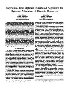
Now, we show that there exists a global node ordering for IC among all nodes in time slot 6. Based on Table III, we can establish a global node ordering for IC among all nodes explicitly. Since none of the primary nodes perform IC, we put active primary nodes p1 , p4 , p8 and p9 in the front of global node ordering list with arbitrary order among them. Based on Bi (t) and Yi (t) in Table III, we can establish a global ordering among the secondary nodes, as shown in Figure 16. The arrows originating from a node in the figure represent the interference from that node. In this figure, we first take a receive node S12 as an example. S12 is being interfered by transmit nodes P1 , S3 and S13 . Since

12

100

S

P12

28

P

100

S21

S

28

90

156

6 S

6

P

S16

S17

5

S14

4

23478 4

70

S24

3

P

S

23

13

60

12

P

8

8

11

134679 S5 1 3 4 6 7 9 S4

20 10

18

P19

P8

S

P

S3

134679 P 16 S 9

17

10

20

30

40

50

S18

S29

P19

S 20

5

10

P18

S4

3 7

S

20

S10

P

S3

20

8

S19

60

70

80

90

S20

P16

S9

S1

P13

S29

P11

S15

S10

P20

P17

S26

0 0

10

20 30 Primary link

0 0

22

S30

11

1

S26

P13

S27

S

P8

S11

30

15

S

P10

40

27

S22

P

S19

S

30

S

2 5 8 10

2 5 8 10

P

1 3 4 6 9 10

S18

S

30

S25

P6

S12

S25

S8

6

2

P10

50

23

P5

P7

S2

S

S13

P1

15

S

S S

P

S7

P14

P

6

14

4

70

2

S

P

S

2578

P7

40

6

5

60 50

S

80

1346

7

14

24

P

16

S17

P2

P1

P15

S

P

S S

3

12

P9

80

90

P

S21 P

9

40

50 60 Secondary link

70

80 90 Interference

100

100

Fig. 14. Routing topology for each primary and secondary sessions and scheduling on each link of the respective route. The numbers in the box next to a link show the time slots when the link is active.

P1 and S3 are before S12 , S12 is responsible for canceling their interference, each with 1 DoF. For the interference from S13 , S12 does not need to use any DoF to cancel this interference, since S13 is after S12 in this global node ordering. This interference is to be canceled by S13 with 2 DoFs. As a second example, consider transmit node S3 . S3 is interfering receive nodes P8 , S5 , S11 and S12 . Since P8 is before S3 , S3 is responsible for canceling this interference with 1 DoF. For its interference to S5 , S11 and S12 , S3 does not need to use any DoF to cancel this interference, since S5 , S11 and S12 are after S3 in this global node ordering. This interference is canceled by S5 , S11 and S12 , respectively, each with 1 DoF. It is easy to verify that based on this global node ordering, the IC responsibilities at nodes S4 , S17 , S24 , S28 , S5 , S11 , S1 , S30 and S13 are all satisfied. C. Comparison to Interweave Paradigm To show the benefits of TC paradigm, we compare our results to those under the interweave paradigm. For the latter, a secondary node is not allowed to transmit (receive) at the same time when a nearby primary node is active. That is, the secondary nodes will not perform inter-network IC for interference to/from the primary nodes. The problem formulation for this paradigm is given in [22], which is similar to the problem formulation for TC paradigm except that we remove DoF allocation by the secondary nodes to cancel interference to/from the primary nodes. The problem formulation remains an MILP, and an upper bound can be obtained by running CPLEX for a given termination time (i.e., 8 hours). Following the same setting as in the case study in the last section, we obtain an upper bound of 0.4 for the objective value (comparing to 0.6 from our distributed solution in Section VI-B). The time slot scheduling on each link of the secondary sessions is shown in Fig. 17. Comparing Fig. 14 and 17, we find that the set of time slots used by each secondary link under interweave paradigm is smaller. We take the link

Fig. 15. Active links in time slot 6 in both primary and secondary networks.

100

S

S28 P9

21

90

P3

6 S6

80

P12

S17

P4

S

24

7 10

S16

5

S14

48

P2

13 70

P1

P15

S

4

P14

P7

60

50

S8

S

9 10

P8

S30

25

8 P10

40

P6 S27

S22

S

S11

P5

S12

6

S2

S23

S13

12

7

18

P13

S29

30

25 1

20

S4

S3

P19

S5

3 9 10

S19

1

8 S26

S15

25 S

3 10

P18

10

P11

P16

3 S20

7

S9

S10

P20

P17

0 0

10

20

30

40

50

60

70

80

90

100

Fig. 17. Routing for each session and scheduling on each link for both primary and secondary networks under the interweave paradigm.

S28 → S17 as an example. Under interweave paradigm, this link cannot use time slot 6 as the neighboring primary link P4 → P9 is using this it. However, under TC paradigm, this link can use time slot 6 to achieve the simultaneous activation with the primary link P4 → P9 . For any secondary link in Figure 17, we cannot find one that simultaneously actives with the primary links. There is no inter-network interference in the network. D. Complete Results We run our distributed algorithm for 50 random network instances, with 20-node primary network and 30-node secondary network. The number of primary and secondary sessions are random, with the source and destination nodes of each session are randomly generated. Table IV compares the objective values from our distributed algorithm and the upper bounds

13

p1

p4

p8

p9 s3

s4

s17 s24

Primary node

Fig. 16.

s28

s12

s5

s11

s1

s30

s13

Secondary node

A global node ordering for IC in time slot 6.

TABLE IV R ESULTS FOR 50 NETWORK INSTANCES . Instance 1 2 3 4 5 6 7 8 9 10 11 12 13 14 15 16 17 18 19 20 21 22 23 24 25

Our Algorithm 0.8 0.7 0.4 0.4 0.4 0.5 0.9 0.7 1.1 0.3 0.6 0.7 0.3 0.9 0.7 1.0 0.9 0.2 0.6 0.6 1.1 0.6 0.8 0.6 0.6

CPLEX

Instance

0.9 0.9 0.5 0.4 0.6 0.6 1.1 0.8 1.1 0.3 0.7 0.8 0.4 1.0 0.8 1.0 1.0 0.4 0.6 0.7 1.1 0.7 0.8 0.9 0.6

26 27 28 29 30 31 32 33 34 35 36 37 38 39 40 41 42 43 44 45 46 47 48 49 50

Our Algorithm 0.7 0.6 0.5 0.5 0.7 1.0 0.8 0.3 0.7 0.5 0.8 0.6 0.5 0.6 0.4 0.6 0.8 0.3 0.5 0.4 0.6 0.8 0.4 0.5 0.8

CPLEX 0.8 0.7 0.7 0.6 0.8 1.1 1.0 0.4 0.9 0.6 0.9 0.8 0.5 0.7 0.4 0.7 0.9 0.3 0.7 0.5 0.6 0.9 0.5 0.6 1.0

from CPLEX solver. The average ratio between the two over 50 instances is 83.7%, with standard derivation of 0.073. Since the optimal objective value (unknown) to the centralized problem lies between the upper bound and the feasible solution obtained by our distributed algorithm, these results affirm that our distributed algorithm is highly competitive.

each node in each iteration of our distributed algorithm. Our distributed algorithm increases the data stream on each active link iteratively based on local computation. Since the nodes in the two local sets of a node directly affect the node’s IC responsibility, our algorithm attempts to switch nodes in the two sets if it can improve the IC structure. Although no explicit node ordering is maintained in our distributed algorithm, we prove that our distributed data structure at each node (with the use of two local sets) can be mapped to an explicit global node ordering for IC among all nodes in the network. This guarantees the existences of feasible precoding/decoding vectors at the secondary nodes to achieve our desired IC in the network (i.e., feasibility at the PHY layer). Through simulation study, we show that our distributed algorithm achieves TC between secondary and primary networks and offers competitive throughput performance when compared to a centralized optimization. ACKNOWLEDGMENTS This work was supported in part by NSF under Grants 1443889, 1343222, 1102013 and ONR under Grant N0001415-1-2926. The work of Dr. S. Kompella was supported in part by the ONR. Part of W. Lou’s work was completed while she was serving as a Program Director at the NSF. Any opinion, findings, and conclusions or recommendations expressed in this paper are those of the authors and do not reflect the views of the NSF. R EFERENCES

VII. C ONCLUSIONS TC is a new spectrum sharing paradigm that allows simultaneous activation of the secondary nodes with the primary nodes. The enabling PHY layer technology for TC is IC, which is the sole responsibility of the secondary nodes. In this paper, we design a distributed algorithm to achieve TC for multihop primary and secondary networks. The main challenge in this algorithm is to ensure that IC is done efficiently (i.e., canceled once by a secondary node) and in a feasible manner (i.e., implementable at the PHY layer). In contrary to a centralized IC algorithm which relies on a global node ordering, we only maintain two local sets for each node to keep track of the node’s IC responsibilities. We show how to establish, maintain, and update these two local sets for

[1] F. Gao, R. Zhang, Y.-C. Liang, and X. Wang, “Design of learningbased MIMO cognitive radio systems,” IEEE Transactions on Vehicular Technology, vol. 59, no. 4, pp. 1707–1720, May 2010. [2] S. Geirhofer, L. Tong, and B.M. Sadler, “Dynamic spectrum access in the time domain: Modeling and exploiting white space,” IEEE Communications Magazine, vol. 45, no. 5, pp. 66–72, May 2007. [3] A. Goldsmith, S.A. Jafar, I. Maric, and S. Srinivasa, “Breaking spectrum gridlock with cognitive radios: An information theoretic perspective,” Proceedings of the IEEE, vol. 97, no. 5, pp. 894–914, May 2009. [4] S. Gollakota and D. Katabi, “Zigzag decoding: Combating hidden terminals in wireless networks,” in Proc. ACM SIGCOMM, pp. 159– 170, Seattle, WA, August 17–22, 2008. [5] Y.T. Hou, Y. Shi, and H.D. Sherali, “Spectrum sharing for multi-hop networking with cognitive radios,” IEEE Journal on Selected Areas in Commun., vol. 26, no. 1, pp. 146–155, Jan. 2008. [6] Y.T. Hou, Y. Shi, and H.D. Sherali, Applied Optimization Methods for Wireless Networks, Cambridge University Press, 2014, ISBN-13: 9781107018808.

14

[7] S. Hua, H. Liu, M. Wu, and S.S. Panwar, “Exploiting MIMO antennas in cooperative cognitive radio networks,” in Proc. IEEE INFOCOM, pp. 2714–2722, Shanghai, China, April. 10-15, 2011. [8] S.K. Jayaweera, M. Bkassiny, and K.A. Avery, “Asymmetric cooperative communication based spectrum leasing via auctions in cognitive radio networks,” IEEE Trans. on Wireless Commun., vol. 10, no. 8, pp. 2716– 2724, August 2011. [9] D. Johnson, Y. Hu, D. Maltz, “The Dynamic Source Routing Protocol (DSR) for Mobile Ad Hoc Networks for IPv4,” IETF RFC 4728, Feb 2007. [10] S.-J. Kim and G.B. Giannakis, “Optimal Resource Allocation for MIMO Ad Hoc Cognitive Radio Networks,” IEEE Transactions on Information Theory, vol. 57, no. 5, pp. 3117–3131, May 2011. [11] R. Manna, R.H.Y. Louie, Y. Li, and B. Vucetic, “Cooperative spectrum sharing in cognitive radio networks with multiple antennas,” IEEE Trans. on Signal Processing, vol. 59, no. 11, pp. 5509–5522, Nov. 2011. [12] C. Perkins, E. Belding-Royer, and S. Das, “Ad hoc on-demand distance vector (AODV) routing,” IETF RFC 3561, July 2003. [13] H. Rahul, S. Kumar, and D. Katabi, “JMB: scaling wireless capacity with user demands,” in Proc. ACM SIGCOMM, pp. 235–246, Helsinki, Finland, Aug. 2012. [14] Y. Shi, J. Liu, C. Jiang, C. Gao, and Y.T. Hou, “A DoF-based link layer model for multi-hop MIMO networks”, IEEE Trans. on Mobile Computing, vol. 13, no. 7, pp. 1395–1408, July 2014. [15] O. Simone, I. Stanojev, S. Savazzi, Y. Bar-Ness, U. Spagnolini, and R. Pickholtz, “Spectrum leasing to cooperating secondary ad hoc networks,” IEEE Journal on Selected Areas in Commun., vol. 26, no. 1, pp. 203–213, Jan. 2008. [16] G.S. Smith, “A Direct Derivation of a Single-Antenna Reciprocity Relation for the Time Domain.” in IEEE Trans. on Antennas and Propagation, vol. 52, no. 6, pp. 1568–1577, June 2004. [17] A.M. Wyglinski, M. Nekovee, and Y.T. Hou, Cognitive Radio Communications and Networks: Principles and Practice. Chapter 12, Academic Press/Elsevier, 2010. [18] X. Xie, X. Zhang, and K. Sundaresan, “Adaptive feedback compression for MIMO networks,” in Proc. of ACM MobiCom, pp. 477–488, Miami, FL, Sep. 2013. [19] X. Yuan, C. Jiang, Y. Shi, Y.T. Hou, W. Lou, S. Kompella, and S.F. Midkiff, “Toward transparent coexistence for multi-hop secondary cognitive radio networks,” IEEE Journal on Selected Areas in Communications, vol. 33, no. 5, pp. 958–971, May 2015. [20] X. Yuan, C. Jiang, Y. Shi, Y.T. Hou, W. Lou, and S. Kompella, “Beyond interference avoidance: on transparent coexistence for multihop secondary CR networks,” in Proc. IEEE SECON, pp. 398–405, New Orleans, LA, June 24–27, 2013. [21] X. Yuan, Y. Shi, Y.T. Hou, W. Lou, S.F. Midkiff, and S. Kompella, “Achieving Transparent Coexistence in a Multi-hop Secondary Network Through Distributed Computation,” in Proc. IEEE IPCCC, Austin, TX, Dec. 5–7, 2014. [22] X. Yuan, X. Qin, F. Tian. Y. Shi, Y.T. Hou, W. Lou, S.F. Midkiff, and S. Kompella, “A Distributed Algorithm to Achieve Transparent Coexistence for a Secondary Multi-hop MIMO Network,” The Bradley Department of Electrical and Computer Engineering, Virginia Tech, Blacksburg, VA, July 2015. URL: https://www.dropbox.com/s/w65ge63ajgori3j/TR20160117%20 with%20appendix.pdf?dl=0. [23] X. Yuan, Y. Shi, Y.T. Hou, W. Lou, and S. Kompella, “UPS: A United Cooperative Paradigm for Primary and Secondary Networks,” in Proc. IEEE MASS, Hangzhou, China, Oct. 14–16, 2013. [24] R. Zhang and Y.-C. Liang, “Exploiting multi-antennas for opportunistic spectrum sharing in cognitive radio networks,” IEEE Journal of Selected Topics in Signal Processing, vol. 2, no. 1, pp. 88–102, February 2008. [25] Y.J. Zhang and A.M.-C. So, “Optimal spectrum sharing in MIMO cognitive radio networks via semidefinite programming,” IEEE Journal on Selected Areas in Communications, vol. 29, no. 2, pp. 362–373, February 2011. [26] J. Zhang and Q. Zhang, “Stackelberg game for utility-based cooperative radio network,” in Proc. ACM MobiHoc, pp. 23–32, New Orleans, LA, USA, May 18–21, 2009. [27] X. Zhang, K. Sundaresan, M.A. Khojastepour, S. Rangarajan, and K.G. Shin, “NEMOx: scalable network MIMO for wireless networks,” in Proc. ACM MobiCom, pp. 453-464, Miami, FL, Sep. 2013. [28] S. Zaks, “Optimal distributed algorithms for sorting and ranking,” IEEE Trans. on Computers, vol. 5, no. 1, pp. 376–379, April 1985.

Xu Yuan (S’13–M’16) received his Ph.D. degree in the Bradley Department of Electrical and Computer Engineering at Virginia Tech, Blacksburg, VA in 2016. His current research interest focuses on algorithm design and optimization for spectrum sharing, coexistence, and cognitive radio networks.

Xiaoqi Qin (S’13) received her B.S. and M.S. degree in Computer Engineering from Virginia Tech in 2011 and 2013, respectively. Since Fall 2013, she has been pursuing her Ph.D. degree in the Bradley Department of Electrical and Computer Engineering at Virginia Tech, Blacksburg, VA. Her current research interest are algorithm design and cross-layer optimization for wireless networks.

Feng Tian (M’13) received his Ph.D. degree in Signal and Information Processing from Nanjing University of Posts and Telecommunications, Nanjing, China in 2008. He is currently an Associate Professor at the same university. He is a visiting scholar at Virginia Tech, USA from 2013-2015. His research focuses on performance optimization and algorithm design for wireless networks.

Yi Shi (S’02–M’08–SM’13) is a Senior Research Scientist at Intelligent Automation Inc., Rockville, MD, and an Adjunct Assistant Professor at Virginia Tech. His research focuses on optimization and algorithm design for wireless networks and social networks. He has co-organized three IEEE and ACM workshops and has been a TPC member of many major IEEE and ACM conferences. He is an Editor of IEEE Communications Surveys and Tutorials. He authored one book, five book chapters and more than 110 papers on wireless network algorithm design and optimization. He has named an IEEE Communications Surveys and Tutorials Exemplary Editor in 2014. He has a recipient of IEEE INFOCOM 2008 Best Paper Award, IEEE INFOCOM 2011 Best Paper Award Runner-Up, and ACM WUWNet 2014 Best Student Paper Award.

Y. Thomas Hou (F’14) is the Bradley Distinguished Professor of Electrical and Computer Engineering at Virginia Tech, Blacksburg, VA. He received his Ph.D. degree from NYU Tandon School of Engineering (formerly Polytechnic Univ.). His current research focuses on developing innovative solutions to complex cross-layer optimization problems in wireless networks. He has published two graduate textbooks: Applied Optimization Methods for Wireless Networks (Cambridge University Press, 2014) and Cognitive Radio Communications and Networks: Principles and Practices (Academic Press/Elsevier, 2009). He is the Steering Committee Chair of IEEE INFOCOM conference and a member of the IEEE Communications Society Board of Governors.

15

Wenjing Lou (F’15) is a professor in the computer science department at Virginia Tech. She received her Ph.D. in Electrical and Computer Engineering from the University of Florida. Her research interests are in the broad area of wireless networks, with special emphases on wireless security and cross-layer network optimization. Since August 2014, she has been serving as a program director at the National Science Foundation. She is the Steering Committee Chair of IEEE Conference on Communications and Network Security (CNS).

Scott F. Midkiff (S’82–M’85–SM’92) is Professor & Vice President for Information Technology and Chief Information Officer at Virginia Tech, Blacksburg, VA. From 2009 to 2012, Prof. Midkiff was the Head of the Bradley Department of Electrical and Computer Engineering at Virginia Tech. From 2006 to 20009, he served as a program director at the National Science Foundation. Prof. Midkiff’s research interests include wireless and ad hoc networks, network services for pervasive computing, and cyber-physical systems.

Sastry Kompella (S’04–M’07–SM’12) received his Ph.D. degree in computer engineering from Virginia Tech, Blacksburg, Virginia, in 2006. Currently, he is the Head of Wireless Network Theory section, Information Technology Division at the U.S. Naval Research Laboratory (NRL), Washington, DC. His research focuses on complex problems in crosslayer optimization and scheduling in wireless and cognitive radio networks.