ACTEA 2009
July 15-17, 2009 Zouk Mosbeh, Lebanon
Application of BP Neural Network in the Prediction of Consolidation Coefficient Hong-Hu ZHU, Student Member, IEEE, Jian-Ping FU and Fei DAI
Abstract—The application of artificial neural network (ANN) in the discipline of geotechnical engineering is discussed in this paper. A multi-layer error back-propagation (BP) feed-forward neural network model was proposed to predict an important geotechnical parameter, namely the consolidation coefficient. The conventional methods for predicting consolidation coefficient is briefly introduced. Based on the results of laboratory consolidation tests, the BP model was trained and used to determine the consolidation coefficient. The predicted values were compared to those determined by graphical methods. It is proved that the BP neural network approach yielded similar results compared with other methods.
I. INTRODUCTION
T
H E theory of artificial neural network (ANN) became a cutting-edge research area in the late 80's around the world and one of the most important branches of artificial intelligence. ANN works like the human brain in simulating biological nervous system, with the following characteristics: (1) It has a giant size; (2) It incorporates parallel processing mechanisms; (3) It has the same fault-tolerant and association capacity as the human brain; (4) It has the ability of self-learning, self-organization and adaptive capacity. Therefore, at present, it is widely used in pattern recognition, image processing, nonlinear optimization, voice processing, natural language understanding, automatic target recognition, robotics and expert systems. In recent years, artificial neural network has been used in the discipline of civil engineering, particularly in the geotechnical field. Because ANN is capable of modeling complex non-linear behavior with high accuracy, it is quite suitable for dealing with practical problems in geotechnical engineering, such as predicting geotechnical parameters. In this paper, a multi-layer error back-propagation feed-forward neural network model (BP neural network,) was used to predict an important parameter in geotechnical engineering, i.e. the consolidation coefficient. The conventional graphical methods used to determine the consolidation coefficient is briefly introduced. Based on laboratory consolidation test results, a BP model was constructed to predict this parameter. The predicted values Manuscript received June 3, 2009. H. -H. Zhu is with Department of Civil and Structural Engineering, The Hong Kong Polytechnic University, Hong Kong, China (phone: 852-2766-6078; fax: 852-2334-6389; e-mail: cehhzhu@ polyu.edu.hk). J. -P. Fu is with Beihang University, Beijing, China (e-mail:
[email protected]). F. Dai is with Department of Civil and Structural Engineering, The Hong Kong Polytechnic University, Hong Kong, China (e-mail:
[email protected]).
978-1-4244-3834-1/09/$25.00 © 2009 IEEE
were compared to those determined by conventional methods. The results showed that the ANN approach yielded high accuracy. II. DETERMINATION OF CONSOLIDATION COEFFICIENT A. Definition of Consolidation Coefficient In Terzaghi’s one-dimensional consolidation theory, the consolidation coefficient is defined as [1] kz Cv = mvγ w (1) where k z is the coefficient of permeability in the vertical direction, γ w is the density of water, m v is the modulus of volume compressibility. The spatial variation of excessive pore water pressure with time and depth is ∂u ∂ 2u (2) = Cv 2 ∂t ∂z For a constant initial hydrostatic excess pore water pressure, the average degree of consolidation U ( t ) over the entire depth of the stratum is ∞ 2 − M 2Tv (3) U (t ) = 1 − ∑ e 2 m =1 M π , Tv = C v t is the time factor related where M = H2 2 (2 m + 1) to the consolidation coefficient C v , the drainage length H and the elapsed time t . There are several methods that can be used to calculated C v , including the log time method [2],[3], the root time method [4],[5], the Scott method [6], the inflection point method [7]–[9], the velocity method [10] the rectangular hyperbola method [11],[12], the slope method [13] and the diagnostic curve method [14]. The first two are the most widely used methods in practice and are considered as standard methods for predicting C v . B. The Log Time Method The log time method was proposed by Casagrande and Fadum (1940) [2]. This method plots the displacement gauge readings against the logarithm of times (see Fig. 1) and makes use of the early and later time responses to determine the point for 50% consolidation, i.e. H2 (4) C v = 0 .197 t 50
443
Authorized licensed use limited to: University of Michigan Library. Downloaded on September 11, 2009 at 11:58 from IEEE Xplore. Restrictions apply.
III. BACK-PROPAGATION NEURAL NETWORK
where t 50 is the time for 50% consolidation. 0.1
1
Time (min) 10 100
1000
10000
Displacement dial gage (cm)
0 Experiment Line 1 0.05
Line 2 U=100% U=50% U=0%
0.1
A. Working Principle The introduction of artificial neural network (ANN) is on basis of scientific research work of modern cranial nerve science. It provides a simplified simulation of the human brain, reflecting some of the basic functions. However, it is not a real description of the human brain. One of the widely accepted definitions of ANN is to utilize available physical devices or computers to simulate some of the structures and functions of an organism’s neural network and, in turn, to be applied in engineering or other fields. The basic element forming ANN is the artificial neuron, generally a multi-input, single-output nonlinear unit, as shown in Fig. 3.
x1
0.15
wi
x2 Fig. 1. Schematic illustration of the log time method.
C. The Root Time Method The root time method was proposed by Taylor (1948) [4]. This method utilized the early time response of consolidation, which theoretically should appear as a straight line in a plot of square root of time versus displacement gauge reading, shown in Fig. 2. The point corresponding to 90% degree of consolidation can be determined by drawing two straight lines DB and DC. Thus the consolidation coefficient can be estimated to be H2 (5) C v = 0 . 848 t 90 where t 90 is the time for 90% consolidation. 0
10
s qr(t) (min) 20
30
40
0 Displacement dial gage (cm)
Experiment Line 1 0.05
Line 2 U=90%
0.1
0.15
Fig. 2. Schematic illustration of the root time method.
It can be seen that, the experiential errors and the interaction of primary and secondary consolidation bring great errors in the determination of consolidation coefficients using the conventional graphical methods.
xj xn- 1
w2 wj ┇ ┇ wn- 1
θ i , ui
yi
wn xn Fig. 3. Schematic illustration of an artificial neural network
For every neuron, the following equation must be satisfied n (6) y i (t ) = f ( ∑ w j x j − θ i ) j =1
where
represent the output of other neurons; w1 , w2 ,..., w n are the transimission weights between other n pieces of neurons and the i th neuron; θ i ( i = 1, 2,..., n ) are the x1 , x 2 ,..., x n
threshold values of the i th neuron; n is the number of inputs; t is time; f is an activation function affected by the threshold values θ1 , θ 2 ,..., θ n ; y i (t ) is the output value of the i th neuron. Neurons aggregates in form of the hierarchical structure. One layer of neurons connected with other layers of neurons in the weighted-neighbor way to form a neural network. According to the connection methods, there are now more than 30 kinds of artificial neural network model has been developed and applied, of which the most representative model is error back-propagation (BP) multi-layer feed-forward neural network. The BP neural network is a kind of multi-layer perceptron network, consisting of an input layer, one or more hidden layers and an output layer. It has been proved that, if the hidden layers of a BP network can be constructed according to the requirements, a three-layer network can achieve the approximation of any continuous function with high accuracy. A standard BP neural network topology is shown in Fig. 4, where LA is the input layer, LB is the hidden layer, LC is the input layer, wi and vi are the connection weights. The learning process of a BP neural network often uses the δ rule, that is, utilization of the known examples of the network as a training
444
Authorized licensed use limited to: University of Michigan Library. Downloaded on September 11, 2009 at 11:58 from IEEE Xplore. Restrictions apply.
set. The criterion of the output layer of the BP neural network is often defined as the error sum of squares of the whole q m training set, i.e. E = 1 ∑ ∑ ( c kj − c j ) 2 . k = 1 j =1
w1j
b1
w1q
cj
wi1 wij ┅
bi
┅
wiq
cq
wpj wpq wp1 bp ┅
vh1 vhp v11 v1i vhi vni vnp v1p vn1 a1 ah an ┅ ┅
a1k
ahk
Lc
Water content 69.0%
w
Unit weight 15.7 kN/m3
Clay
Liquid limit: 51.2%
Silt
Plastic limit: 25.2%
Sand
Gravel
100
LB v LA
ank
80 60 40 20
Fig. 4. Standard topological structure of a BP network.
0 0.0001
0.001
0.01
0.1
1
10
Grain size (mm)
p0 , and the consolidation pressure p . Thus in the BP model, these three parameters were chosen as the input parameters.
Fig. 5. Typical gradation curves of Guangzhou marine clay
In the BP model, the hyperbolic tangent activation function was used in the hidden layer. The linear
f1 = ( e n − e − n ) / ( e n + e − n )
function f1 = n was used in the output layer. In the training phase, the results of the first 18 tests, i.e. 72 training samples, were used. The actual consolidation coefficients were considered to be the values determined by the log time method. The trained BP model was then used to predict the consolidation coefficients in the last 2 consolidation tests. V. RESULTS The comparison of predicted consolidation coefficient by the BP model, the log time method and the root time method are shown in Fig. 6. The results indicate that the BP model has the ability to predict the consolidation coefficient like conventional graphical methods. 30
30
25
25
20
20
15
15
10
10
5
5
-4
2
(10 cm /s)
Geotechnical engineering is a very practical field. Many of the geotechnical parameters are determined by laboratory and field testing, or just past experiences. The BP neural network starts directly from the measured samples (as the training set) and ends with the prediction of parameters, which minimizes the artificial errors. More importantly, the accuracy of BP networks can be improved automatically with the increase of samples. Therefore, the BP neural network has been increasingly used in geotechnical engineering [15]–[18]. To construct a BP neural network model to predict the consolidation coefficient, a series of consolidation tests were conducted in laboratory. The soil specimens used in this study was taken from Nansha Development Zone (NDZ) of Guangzhou, China. NDZ is located on the west coast of the Lingding Sea that connects both Hong Kong and Macau and is geographical center of the Pearl River Delta. The specimens were dark grey in color and kept in an undisturbed state. The basic physical and mechanical properties are shown in Table 1. The typical gradation curves for Guangzhou marine clay (GMC) are given in Fig. 5. Twenty consolidation tests were carried out on Casagrande-type oedometers under a double drainage condition. The diameter and height of the specimens were 60 mm and 20 mm, respectively. The specimens were loaded to 50kPa, 100kPa, 200kPa and 400kPa in stages. For each stage, the loading was kept for 1 day to ensure the primary consolidation was completed. Previous studies shows that the consolidation coefficient is affected by initial void ratio e0 , the preconsolidation pressure
Predicted Cv by theBP model__
IV. MATERIALS AND METHODS
0
2
w11
┅
Specific gravity 2.71
-4
c1
TABLE I BASIC PROPERTIES OF GUANGZHOU MARINE CLAY
cq k
method_ (10 cm /s)
cjk
Predicted Cv by the root time_
c1k
Percent finer by weight
2
The output parameter was consolidation coefficient.
0 0
5
10
15
20
25 -4
30
2
Predicted Cv by the log time method (10 cm /s)
Fig. 6. Comparison of predicted consolidation coefficients by the BP model, the log time method and the root time method
445
Authorized licensed use limited to: University of Michigan Library. Downloaded on September 11, 2009 at 11:58 from IEEE Xplore. Restrictions apply.
VI. CONCLUSION Recently, neural networks have been more and more widely used in geotechnical engineering. This approach has shown excellent ability to cope with indefinable and complicated problems. In this paper, neural networks are used to predict an important geotechnical parameter, namely consolidation coefficient. On the basis of experimental data, a back-propagation neural network model was developed to determine consolidation coefficient. In this model, the initial void ratio, the preconsolidation pressure, and the consolidation pressure were chosen as the inputs. The performance of this model shows high accuracy compared with conventional graphical methods. However, it should be noted that adequate measurements should be used to train the BP neural network model, so as to improve its reliability. REFERENCES [1] [2] [3] [4] [5] [6] [7] [8] [9] [10] [11] [12] [13] [14] [15] [16] [17] [18]
K. Terzaghi, R.B. Peck, G. Mesri, Soil mechanics in engineering practice. 3rd ed. New York: Wiley, 1996. A. Casagrande, R. C. Fadum, “Notes on soil testing for engineering purposes,” Soil Mechanics Series No. 8, Publication No.268, Harvard Univ., Cambridge, Mass., 37. 1940. R.G. Robinson, M. M. Allam, “Determination of coefficient of consolidation from early stage of log t plot,” Geotech. Test. J., vol. 19, no. 3, pp. 316–320, 1996. D. W. Taylor, Fundamentals of soil mechanics. New York: Wiley, 1948. T. W. Feng, Y. J. Lee, “Coefficient of consolidation from the linear segment of the t1/2 curve,” Can. Geo. J., vol. 38, no.4, pp. 901–909, Aug. 2001. R. F. Scott, “New method for consolidation-coefficient evaluation,” J. Soil Mech. and Found. Div., vol. 87, no. 1, pp. 29–41, 1961. F. R. Cour, “Inflection point method for computing Cv,” J. Soil Mech. and Found. Div., vol. 97, no. 5, pp. 827–831, 1971. R. G. Robinson, “Consolidation analysis by an inflection point method,” Géotechnique, vol. 47, no. 1, pp.199–200, 1997. G. Mesri, T.W. Feng, M. Shahien, “Coefficient of consolidation by inflection point method,” J. Geotech. Geoenviron. Eng., vol. 125, no. 8, pp.716–718, 1999. A. K. Parkin, “Coefficient of consolidation by the velocity method,” Géotechnique, vol. 28, no. 4, pp. 472–474, 1978. A. Sridharan, A. S. Rao, “Rectangular hyperbola fitting method for one-dimensional consolidation,” Geotech. Test. J., vol. 4, no. 4, pp. 161–168, 1981. A. Sridharan, N.S. Murthy, K.Prakash, “Rectangular hyperbola method of consolidation analysis,” Géotechnique, vol. 37, no. 3, pp. 355–368, 1987. M. S. Al-Zoubi, “Coefficient of consolidation by the slope method,” Geotech. Test. J., vol.31, no.6, pp. 1–5, Nov. 2008. S. K. Singh, “Diagnostic curve methods for consolidation coefficient,” Int. J. Geomechanics, vol. 7, no. 1, pp. 75–79, Feb. 2007. F. Mayoraz, L. Vulliet, “Neural networks for slope movement prediction,” Int. J. Geomechanics, vol. 2, no. 2, pp. 153–173, 2002. Y. Yang, M. S. Rosenbaum, “The artificial neural network as a tool for assessing geotechnical properties,” Geotech. Geol. Eng., vol. 20, no. 2, pp. 149–168, 2002. S. Celik, O. Tan, “Determination of preconsolidation pressure with artificial neural network,” Civil Eng. Environ. Sys., vol. 22, no. 4, pp. 217–231, 2005. M. A. Shahin, M. B. Jaksa, H. R. Maier, “State of the art of artificial neural networks in geotechnical engineering,” Electron. J. Geotech. Eng., pp.1–26, 2008.
446
Authorized licensed use limited to: University of Michigan Library. Downloaded on September 11, 2009 at 11:58 from IEEE Xplore. Restrictions apply.