Neuron, Volume 92
Supplemental Information
Computational Precision of Mental Inference as Critical Source of Human Choice Suboptimality Jan Drugowitsch, Valentin Wyart, Anne-Dominique Devauchelle, and Etienne Koechlin
Computational precision of mental inference Drugowitsch, Wyart, Devauchelle, and Koechlin
Supplemental Information
Contents 1
Supplemental Figures
2
2
Supplemental Experimental Procedures 2.1 Stimulus and task design details . . . . . . . . . . . . . . . . . . . . . . . . . . . . . 2.2 Optimal decision making without added variability . . . . . . . . . . . . . . . . . . 2.2.1 Generative model . . . . . . . . . . . . . . . . . . . . . . . . . . . . . . . . . . 2.2.2 Optimal decision-making . . . . . . . . . . . . . . . . . . . . . . . . . . . . . 2.3 Introducing variability . . . . . . . . . . . . . . . . . . . . . . . . . . . . . . . . . . . 2.3.1 Variability at the selection stage . . . . . . . . . . . . . . . . . . . . . . . . . . 2.3.2 Variability at the inference stage . . . . . . . . . . . . . . . . . . . . . . . . . 2.3.3 Variability at the sensory stage . . . . . . . . . . . . . . . . . . . . . . . . . . 2.3.4 Variability at the prior stage . . . . . . . . . . . . . . . . . . . . . . . . . . . . 2.3.5 Variability at multiple stages . . . . . . . . . . . . . . . . . . . . . . . . . . . 2.3.6 Misspecification of subjective generative concentration κ . . . . . . . . . . . 2.4 Decomposing variability into deterministic biases and residual terms . . . . . . . . 2.4.1 The bias-variance decomposition . . . . . . . . . . . . . . . . . . . . . . . . . 2.4.2 Estimating the contribution of deterministic biases to the overall variability 2.5 Introducing explicit temporal and spatial biases . . . . . . . . . . . . . . . . . . . . 2.5.1 Spatial biases . . . . . . . . . . . . . . . . . . . . . . . . . . . . . . . . . . . . 2.5.2 Temporal biases . . . . . . . . . . . . . . . . . . . . . . . . . . . . . . . . . . . 2.6 The relation between the softmax and the cumulative Gaussian . . . . . . . . . . . 2.6.1 Gaussian noise . . . . . . . . . . . . . . . . . . . . . . . . . . . . . . . . . . . 2.6.2 Gumbel-distributed noise . . . . . . . . . . . . . . . . . . . . . . . . . . . . . 2.6.3 Relating Gaussian and Gumbel-distributed noise . . . . . . . . . . . . . . . 2.7 Sensory variability choice distributions . . . . . . . . . . . . . . . . . . . . . . . . . 2.7.1 Choice distribution for 2-categories condition . . . . . . . . . . . . . . . . . 2.7.2 Choice distribution for 3-categories task . . . . . . . . . . . . . . . . . . . . . 2.7.3 Accuracy of the Gaussian approximation . . . . . . . . . . . . . . . . . . . . 2.7.4 The relation between sensory and inference variability . . . . . . . . . . . . 2.8 Choice distributions with deterministic biases . . . . . . . . . . . . . . . . . . . . . 2.8.1 Choice distribution for the 2-categories condition . . . . . . . . . . . . . . . 2.8.2 Choice distribution for the 3-categories condition . . . . . . . . . . . . . . . 2.8.3 Fitting models with deterministic biases . . . . . . . . . . . . . . . . . . . . . 2.8.4 The contribution of sequential biases . . . . . . . . . . . . . . . . . . . . . . . 2.8.5 Stability of deterministic biases . . . . . . . . . . . . . . . . . . . . . . . . . . 2.9 Model fitting, fit validation, and number of parameters . . . . . . . . . . . . . . . . 2.9.1 Validating the model fitting procedure . . . . . . . . . . . . . . . . . . . . . . 2.9.2 Number of parameters . . . . . . . . . . . . . . . . . . . . . . . . . . . . . . . 2.10 Computing the information loss for the 2-categories condition . . . . . . . . . . . .
1
. . . . . . . . . . . . . . . . . . . . . . . . . . . . . . . . . . . .
. . . . . . . . . . . . . . . . . . . . . . . . . . . . . . . . . . . .
. . . . . . . . . . . . . . . . . . . . . . . . . . . . . . . . . . . .
. . . . . . . . . . . . . . . . . . . . . . . . . . . . . . . . . . . .
. . . . . . . . . . . . . . . . . . . . . . . . . . . . . . . . . . . .
. . . . . . . . . . . . . . . . . . . . . . . . . . . . . . . . . . . .
10 10 11 11 11 12 12 12 13 14 14 14 16 16 17 19 19 19 22 22 22 23 25 25 26 26 27 28 28 29 31 31 32 33 33 34 35
Computational precision of mental inference Drugowitsch, Wyart, Devauchelle, and Koechlin
1
Supplemental Information
Supplemental Figures
List of Figures S1 S2 S3 S4 S5 S6 S7
Psychometric functions and variability for different trial subgroups . . . . . . Recovering model parameter fits and estimates from simulated behavior . . . Illustrating and validating model assumptions and approximations . . . . . . Deterministic biases and fraction match for different trial subgroups . . . . . Spatial and temporal biases . . . . . . . . . . . . . . . . . . . . . . . . . . . . . Model comparison with biases . . . . . . . . . . . . . . . . . . . . . . . . . . . Lapse and response bias parameters for model assuming inference variability
2
. . . . . . .
. . . . . . .
. . . . . . .
. . . . . . .
. . . . . . .
. . . . . . .
. . . . . . .
. . . . . . .
. . . . . . .
3 4 5 6 7 8 9
Computational precision of mental inference Drugowitsch, Wyart, Devauchelle, and Koechlin
A
first half of trials
second half of trials 1.0
mal
fraction correct
pti Bayes-o
0.8
0.6 2
B
4
6
8
10
12
14
sequence length
pti Bayes-o
0.6 2
4
following correct choices 1.0
0.8
0.6 6
8
10
12
sequence length
C
14
10
12
14
16
ptimal Bayes-o
0.8
0.6
16
2
2 categories σinf, 2nd half
8
1.0
ptimal
4
6
sequence length following errors
Bayes-o
2
mal
0.8
16
fraction correct
fraction correct
1.0
fraction correct
Supplemental Information
4
6
8
10
12
sequence length
14
16
3 categories
1
0
ρ�0.75, p<104 0
1
ρ�0.88, p<106 0
1
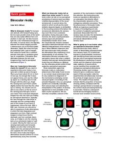
σinf, 1st half Figure S1. Relates to Figure 2. Psychometric functions and variability for different trial subgroups. (A) Left panel: psychometric function for the two-category condition of exp. 1 (orange) and 3 (green) in the first half of trials. Right panel: psychometric function for the two-category condition of exp. 1 and 3 in the second half of trials. (B) Left panel: psychometric function for the two-category condition of exp. 1 and 3 in trials following correct choices. Right panel: psychometric function for the two-category condition of exp. 1 and 3 in trials following errors. In both (A) and (B) error bars indicate s.e.m., and the black curve indicates the theoretical psychometric function of the normative, Bayes-optimal observer. Due to the lower number of available trials, we did not include the data and fits from experiment 2. (C) The two panels show for each subject the inferred variability magnitude (mode ± 95% credible intervals) when fitting the inference variability model to either only the first half or the second half of all trials of the first experiment. In no case was there a significant difference across subjects between the variability magnitude for the two trial subgroups (2 categories, t21 = 1.1, p = 0.3; 3 categories, t21 = 0.5, p = 0.6). In both cases, the inferred magnitude was significantly correlated across trial subgroups (ρ and p in plots denote Pearson product-moment correlation coefficient statistics).
3
Computational precision of mental inference Drugowitsch, Wyart, Devauchelle, and Koechlin 3 categories
estimated σinf
0
true (simulated) σinf
sensory
1
0
1
0
0.1
0.2
0
inference
C
selection
0.6 0.4 0.2 sen
D
inf
source
sel
2 categories
Bayes factor
1
0
pexc > 0.99
sen
inf
sel
0
0
0
0
1
true (simulated) σinf
0.1
0.2
0
3 categories
1
0
0
true (simulated) p(lapse)
0
1
true (simulated) fraction biases
1
0
0
1
true (simulated) fraction biases
model fits to simulated sources of heavy-tailed choice variability inference pexc > 0.99
sen
inf
sel
100
3 categories
selection
sensory
pexc > 0.99
sen
inf
sel
1
0 200
pexc > 0.99
sen
inf
inference pexc > 0.99
selection pexc > 0.99
sel
100
50 0
-50
1
2 categories
p(model)
p(model)
sensory
2 1
true (simulated) p(lapse)
0.8
0
1
1
estimated fraction biases
0
avg. across subjects
2
Bayes factor
fraction choice variability explained
B
1
1
1 0
2
estimated σinf
1
2
estimated p(lapse)
avg. across subjects
estimated p(lapse)
2 categories
estimated fraction biases
A
Supplemental Information
0
-100
log10
0 1 fraction of simulations model deemed best
log10
0 1 fraction of simulations model deemed best
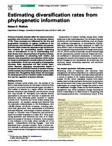
Figure S2. Relates to Figures 3, 5, and 6. Recovering model parameter fits and estimates from simulated behavior. (A) To test how well we could distinguish between inference variability and random lapses, we simulated subject behavior assuming inference variability on the exact same trials that the humans subjects saw in the first experiment. To see how well we recover either of the two parameter, we varied one parameter while keeping the other constant. Per parameter combination we simulated behavior separately for each of the 22 subjects, and computed mean parameter estimates across subjects for 1000 repetitions of this procedure (showing mean, error bars = 2.5th to 97th percentile across repetitions). The dashed lines (mostly below the estimated values) show the true parameter values used for the simulations. For both conditions, there is a ”spill-over” between the estimated variability and lapse rate, but this bias is negligible for parameter ranges that we recover from fitting the human subject data (grey lines). (B) To validate the variability decomposition, we applied the same procedure as in (A), but this time performed for each of the 22 subjects three simulations, each introducing variability at a different point in the decision-making process (sensory/inference/selection; indicated by top labels). The magnitude of this variability was set to match the human subjects’ observed performance. The results show means and SDs across 1000 repretitions of this procedure, using the exact same procedure as for Fig. 5A in the main text to compute the variability decomposition, but this time on the simulated behavior. (C) To test how well we could distinguish deterministic biases from unstructured variability, we simulated behavior with variability due to inference and deterministic biases according to the model described in Sec. 2.8. The behavior was simulated for the exact same trial sequences observed by the 18 human subjects performing the third experiment. The plots show the estimated average fraction of deterministic biases across subjects (mean, error bars from 2.5th to 97.5th percentile across 1000 repetitions) when fitting our model to simulated behavior. The plots illustrate that, in particular for the range of fractions observed for human subjects (around 0.3), the model correctly recovers the correct fraction. (D) To test how sensitive our model fits are to assuming Gaussian inference variability, we here repeated the analysis of Fig. 3A (main text) described in Sec. 2.9.1, while using heavy-tailed Student’s T distributed inference variability with 2.5 degrees of freedom (df ) to simulate the behavior, while still assuming Gaussian variability when fitting the different models. df > 2 was chosen to have a well-defined mean and variance. 4
Computational precision of mental inference Drugowitsch, Wyart, Devauchelle, and Koechlin
spatial biases
B
both biases
−10
0
x
p(choice), simulation
10
−10
0
0
10
−10
D
1
p(x=1|z1-z2)
C
fk(θnt)-fj(θnt)
0.999 0.90 0.50 0.10 0.001
logistic sigmoid cumulative Gaussian −2
−1
0
z1-z2
1
2
mutual information (bits)
p(fk(θnt)-fj(θnt)
p(fk(θnt)-fj(θnt))
temporal biases
0
1
0
2 categories
0
noisy noise-free
0
1
0
1
10
0.1
0
3 categories
p(choice), model
1
noise SD due to inference
2
fraction information loss
A
Supplemental Information
1 0.8 0.6 0.4 0.2 0
0
1
noise SD due to inference
2
Figure S3. Relates to Figure 6. Illustrating and validating model assumptions and approximations. (A) Here we show by simulation that temporal and spatial biases from Sec. 2.5 cause the bias term differences fj (θnt ) − fk (θnt ) to roughly follow a zero-mean Gaussian distribution, as assumed in in Sec. 2.4. The above shows their empirical distribution, found by simulating 105 trials with different sample sequences, as observed by subjects in the three-category condition of the first experiment. For each trial, we computed the contribution of each sample to the log-posteriors while adding the temporal and/or spatial biases discussed in Sec. 2.5, with parameters γθ = 5◦ , γκ = 1, γc = 0.1 (spatial biases), and αa = e−0.1 , αb = 0.01 (temporal biases). Denoting these biased contributions by `ˆntk (including their temporal weighting and spatial perturbation) and their � � unbiased counterparts by `ntk , we found for each sample θnt in each trial n the bias difference by fk (θnt ) − fj (θnt ) = `ˆntk − `ˆntj − (`ntk − `ntj ) for each k 6= j. The distribution of differences is shown from left to right for temporal biases and spatial biases only, and for both biases in combination. The top panels of (A) show the histogram of differences and the best-fit zero-mean Gaussian (arbitrarily scaled). The bottom panel show the cumulative data distribution in grey, scaled vertically such that the cumulative of a Gaussian becomes a line. The black line connects the 1st and 3rd quantile. The figure shows that, except for the tails, fk (θnt ) − fj (θnt ) is well approximated by a Gaussian. (B) To test if the Gaussian approximation for the sensory variability model did not strongly perturb the derived choice probabilities, we compared the choice probabilities computed with the approximate expressions to those found by simulation. Assuming σsen = 30◦ (= π/6 radians), we tested the match on 500 typical trials, by, for each trial, simulating 50.000 instantiations of the sensory noise to get an empirical estimate of these choice probabilities. In each trial we computed one choice probability per category, each corresponding to a different color in the above plots. We deliberately chose a very high noise magnitude, as in this noise regime the Gaussian approximation is more likely to break down. (C) To illustrate the similarity between the logistic sigmoid and the cumulative Gaussian, we here plot the cumulative function of a zero-mean Gaussian with unit variance, and the matching logistic sigmoid with β determined by Eq. (S44). The variance of the Gaussian results from the difference of two Gaussian variables with individual variances σ 2 = 12 . The latter is the variance used to compute β. (D) The left panel shows the mutual information between the sample log-likelihood ratio and the generative category for the noisy and noise-free log-likelihood ratio for a single stimulus orientation (see Sec. 2.10 for the derivation). In the noise-free case, this mutual information is approximately 0.085 bits per oriented stimulus (1 bit = revealing correct category). In the noisy case, the mutual information drops monotonically with the standard deviation of the noise, matching the noise-free case only for σinf = 0. The right panel shows the fraction information loss of the noisy case when compared to the noise-free case. This information loss is computed as one minus the ratio between noisy and noise-free mutual information, as shown in (A). At σinf = 2, this loss reaches above 0.9, indicating that at this level of variability, less than 10% of the original information remains.
5
Computational precision of mental inference Drugowitsch, Wyart, Devauchelle, and Koechlin
fraction match
C
1
0.85 0.8
16
14
12
10
8
6
2 categories
all trials 1st half 2nd half
1
16 14 12
10
8
6
−90 −60 −30 0
0.85 0.8
all trials close pairs distant pairs
0.7
30 60 90
sample tilt (deg)
1
0
samples from choice
0.7 0.65
16
14
12
10
8
6
0.55
l l h e non emporaspatia bot t
1 0
−1 −90 −60 −30 0
3 categories
all trials 1st half 2nd half
30 60 90
sample tilt (deg)
1 0
samples from choice
0.6
0.75
l l e h non emporaspatia bot t sequence perturbation(s)
0
following errors log-likelihood (arb.)
30 60 90
sample tilt (deg)
0
1
−1
−90 −60 −30 0
samples from choice
0.75 0.7
0
sample weight (arb.)
−90 −60 −30 0 30 60 90 sample tilt (deg)
0
1
−1
−1
following correct choices
sample weight (arb.)
0
log-likelihood (arb.)
1
B
second half of trials
sample weight (arb.)
sample weight (arb.)
log-likelihood (arb.)
first half of trials
log-likelihood (arb.)
A
Supplemental Information
0.7 0.65
16
14
12
10
8
6
samples from choice
all trials close pairs distant pairs
0.6
l l e h non emporaspatia bot t
0.55
l l e h non emporaspatia bot t
Figure S4. Relates to Figure 7. Deterministic biases and fraction match for different trial subgroups. (A) Left panel: feature (top row) and temporal (bottom row) encoding curves for the two-category condition of exp. 1 in the first half of trials. Right panel: feature (top) and temporal (bottom) encoding curves for the two-category condition of exp. 1 in the second half of trials. (B) Left panel: feature (top row) and temporal (bottom row) encoding curves for the two-category condition of exp. 1 in trials following correct choices. Right panel: feature (top) and temporal (bottom) encoding curves for the two-category condition of exp. 1 in trials following errors. In (A) and (B), dots and error bars indicate human data and s.e.m., and curves and shaded error bars indicate best-fitting model predictions including feature (top) and temporal (bottom) deterministic biases. (C) Fraction matched choices for trial subgroups, experiment 3. The fraction of matched choices (± SEM across subjects) are compared for paired trials when computed across all trials (thick bars) to the fraction computed for trial subgroups (thin bars) for different trial pairings (none = exact same sample sequence, temporal = one trial is shuffled version of other, spatial = one trial is mirrored version of other, both = temporal + spatial). On one hand (left panels), we computed this fraction match for the first and second half of trials separately, while excluding trial pairs that spun both trial subgroups. On the other hand (right panels), we split trial pairs into those that appeared closer together within the trial sequence, and those that were more distant. In no case did we find a significant effect of trial sub-grouping on the measured fraction of matched choices (2-way repeated-measures ANOVAs, 1st/2nd half, 2 categories: trial subgroup F1,17 = 1.2, p = 0.3, perturbation F3,51 = 14.7, p < 0.001, trial subgroup × perturbation F3,51 = 1.0, p = 0.4; 3 categories: trial subgroup F1,17 = 0.1, p = 0.74, perturbation F3,51 = 18.6, p < 0.001, trial subgroup × perturbation F3,51 = 0.8, p = 0.5; close/distant pairs, 2 categories: trial subgroups F1,17 = 0.3, p = 0.6, perturbation F3,51 = 27.8, p < 0.001, trial subgroups × perturbation F3,51 = 1.4, p = 0.3; 3 categories: trial subgroups F1,17 = 0.4, p = 0.5, perturbation F3,51 = 30.6, p < 0.001, trial subgroups × perturbation F3,51 = 0.4, p = 0.8).
6
Computational precision of mental inference Drugowitsch, Wyart, Devauchelle, and Koechlin
Supplemental Information
Spatial biases
A
B
1
0
log-likelihood
log-likelihood
1
-10º 0º
10º −1
−90
−60
−30
0
30
60
0
0
0.2 −1
90
-0.2
−90
−60
stimulus orientation (deg) biased stimulus orientation (deg)
C log-likelihood
1
0 -1 0 1 −1
−90
−60
−30
0
30
0
30
60
90
60
90
90
0
−90 −90
0
90
true stimulus orientation (deg)
stimulus orientation (deg)
Temporal biases
E
D
1
temporal weight
temporal weight
−30
stimulus orientation (deg)
1 0.80 0.90 0.95 1.00 1.02
0.5
14
12
10
8
6
4
2
0
0.5
14
number of stimuli before last
12
10
8
6
4
2
0
number of stimuli before last
Figure S5. Relates to Figures 6 and 7. Spatial and temporal biases. (A) illustrates the orientation bias for different values of γθ , causing a shift in the log-likelihoods. (B) shows the change in log-likelihoods due to the confirmation bias for different values of γc . (C) illustrates both the change in log-likelihoods (right panel) and the biased stimulus orientation (left panel) due to the oblique effect for different values of γκ . In these panels, the different colors correspond to different categories in the 3-categories condition, and the saturation of these colors to different parameter values. Panels (D) and (E) show the weight λnt applied to the log-likelihood of samples at different points within the samples sequence, aligned to the last sample in this sequence. (D) shows the temporal bias introduced by time-invariant exponential weighting for different values of the parameter α. As can be seen, α < 1 introduces a recency effect, and α > 1 a primacy effect. (E) shows the bias for the linearly changing exponential weighting scheme with parameters αa = 0.85 and αb = 0.01. The different shadings correspond to weightings of sequences of different lengths, and illustrate that introducing a linear dependency in the trial-by-trial weighting causes the overall weighting to depend on the sequence length.
7
Computational precision of mental inference Drugowitsch, Wyart, Devauchelle, and Koechlin
A
Supplemental Information
D
3 categories
0.0
assigned source of choice variability sensory prior likelihood accum. selection 2 categories
choice variability (llh2)
choice variability (llh2)
assigned source of choice variability sensory prior likelihood accum. selection 2 categories
0.0
4 8 12 16
3 categ.
1 p�0.8693
0 0
p�0.9972
senpri llh ac sel
0
senpri llh ac sel
−40 −80
C
2 categ.
3 categ.
sen pri ac sel
sen pri ac sel
p�0.9684
0
E
Bayes factor p(model family)
Bayes factor p(model family)
2 categ.
p>0.9999
0
−40 log10
−200
4
8
12
sequence length
sequence length
B
3 categories
log10
−80
log10
−200
log10
2 categ.
3 categ.
1 p�0.5101
0 0 −50
p�0.9391
senpri llh ac sel
log10
F
0
−100
senpri llh ac sel
log10
2 categ.
3 categ.
p�0.8917
0 −50
p�0.9969
sen pri ac sel
log10
0
−100
sen pri ac sel
log10
Figure S6. Relates to Figures 3 and 4. Model comparison for different variability models, taking into account temporal and spatial biases. This figure differs from Fig. 3A/B in the main text in that it is based on models with temporal and spatial biases. Panels (A)-(C) shows the comparison based on the data of experiment one, and (D)-(F) based on that of experiment three. Taking into account these biases does not change our main conclusions. We considered all possible bias combinations, resulting in 24 models per variability type. The use of temporal biases allows us to distinguish between prior and selection variability (see Sec. 2.3.4) (A)/(D) Model prediction (grey line and shaded area, mean ± SEM across subjects) vs. per-sequence length fit (dots with error bars, mean ± SEM across subjects) of how the noise variance changes with sequence length for five variability models and both task conditions. These predictions are shown for each variability type for the combination of biases that best fitted the subjects’ behavior. The larger number of parameters of models with biases resulted in a better per-subject fit, but in a larger across-subject variability in the fitted parameters, as reflected by the larger error bars than in Fig. 3A in the main text. (B)/(E) FFX and RFX model comparison for different models and conditions. The RFX comparison (top) compares model families, where each family features all models of a specific variability type with all possible combinations of spatial and temporal bias (sen = sensory, pri = prior, llh = likelihood, ac = accumulation, sel = selection; mean probability ± SD). The exceedance probability p is the probability with which the likelihood variability model family is more likely than any other model family. The FFX comparison (bottom) shows for each variability model family the Bayes factor for each family compared to the accumulation variability family. This factor is based on the model within each family with the highest model evidence. The grey line at 210 = 100 is the threshold at which the evidence in favor of the accumulation model is considered decisive. (C)/(F) Same as (B)/(E), but without the likelihood variability model family. This comparison was included to avoid the sharing of probability mass between too-similar models (Stephan et al., 2009).
8
Computational precision of mental inference Drugowitsch, Wyart, Devauchelle, and Koechlin
B
3 categories 2
sorted subjects
sorted subjects
2 categories
response bias 2
A
Supplemental Information
0
0.1
lapse probability
0.2 −2
0
response bias
2
0
0.1
lapse probability
0.2
0
−2 −2
0
response bias 1
2
Figure S7. Relates to Figure 3. Lapse and response bias parameters for model assuming inference variability. All panels show parameter modes ± 95% credible intervals per subject. The subjects are not aligned across panels. (A) Lapses and biases for the 2-categories condition of the first experiment. The left panel shows the lapse probability per subject (mode across subjects not significantly different from zero, t21 = 1.9, p = 0.075). The right panel shows the response bias added to category 1 per subject (mode across subjects not significantly different from zero, t21 = −1.7, p = 0.099). (B) The same as in (A), but for the 3-categories condition. The right panel shows the response biases added to categories 1 and 2 per subject. Across subjects, the mode of only the lapse probability is marginally different from zero (lapse probability, t21 = 2.1, p = 0.022; response bias 1, t21 = −1.5, p = 0.14; response bias 2, t21 = 0.6, p = 0.6).
9
Computational precision of mental inference Drugowitsch, Wyart, Devauchelle, and Koechlin
2
Supplemental Information
Supplemental Experimental Procedures
Section 2.1 provides additional details about the stimulus and task. Sections 2.2 to 2.5 provide further details about used models. All sections from Section 2.6 onwards provide more in-depth mathematical details, but are not required reading to understand the essence of the models.
2.1
Stimulus and task design details
Stimuli were high-contrast, noise-free Gabor patterns (diameter: 4 degrees of visual angle, spatial frequency: 2 cycles per degree of visual angle, Michelson contrast: 75%) of varying orientation, presented at fixation for 100 ms at an average stimulation rate of 3 Hz with small amount of uniform jitter (±33 ms). Sequence lengths (i.e., the number of stimuli per sequence) varied uniformly and unpredictably from 2 to 16 stimuli. Each Gabor pattern was presented on top of a luminance pedestal, and each sequence began with two luminance pedestals presented in rhythm with the following Gabor patterns so that the onset of the first stimulus was predictable in time. At sequence offset, participants were prompted by a luminance pedestal in the fixation point (go signal) for a choice regarding the most likely generative category of the sequence. Participants provided their response by pressing one out of two (or three, depending on the condition) keys with their right hand. The mapping between categories (represented as colors) and response keys was fixed and explained to the participant before the start of the experiment. If no response was provided 1 s following the go signal, the trial was aborted and the participant was informed by a beep that his response was too slow which represented less than 1% of trials for all tested participants. Following each response, feedback about the true generative category of the sequence was provided via a transient change in the color of the fixation point (e.g., from grey to pink if the sequence was generated from the pink category). We did not provide feedback as to whether participants picked the most likely category given the limited evidence provided by the sequence. Consequently, as in the weather prediction task, participants accuracy was bounded by the randomness of presented sequences around their generative means. Furthermore, this means that participants could learn not only the means, but also the spreads of generative distributions.
10
Computational precision of mental inference Drugowitsch, Wyart, Devauchelle, and Koechlin
Supplemental Information
2.2
Optimal decision making without added variability
2.2.1
Generative model
The generative model of the task is as follows. In each trial n of N independent trials, the experimenter picks one category k ∈ {1, . . . , K} (called decks in the main text; K ∈ {2, 3} for 2 or 3 categories) with associated category mean µk . Based on this mean, Tn orientations, θn1 , . . . , θnTn , called samples (or cards in the main text), are generated by drawing them independently and identically distributed (i.i.d.) from a von Mises distribution over the half-ciricle [0, π), centered on µk and with concentration κ. That is, each sample is independently drawn from eκ cos(2(θnt −µk )) p (θnt |µk ) = , (S1) πI0 (κ) where I0 (·) is the modified Bessel function of order 0. 2.2.2
Optimal decision-making
To derive the optimal decision-making strategy, we assume a uniform prior over categories, and a 0-1 loss function, charaterized by a gain (loss) of 0 (1) for correct (incorrect) decisions. For such a loss structure, it is optimal to choose the option associated with the most likely generative category (Berger, 1993). To find this most likely category, we assume subjects to know the category means, µ1 , . . . , µK , and the concentration parameter κ of the generative density, Eq. (S1). Based on this and the uniform category prior, p(µk ) ∝ 1, the posterior probability of category k having generated θn1:Tn = {θn1 , . . . , θnTn } in trial n is by Bayes rule, p(µk |θn1:Tn ) ∝ p(θn1 , . . . , θnTn |µk ) =
Tn Y
p(θnt |µk ).
(S2)
t=1
If xn denotes the chosen category in trial n, then optimal decision-making is performed by choosing the xn = k for which the above posterior is a maximum, that is xn = argmaxk p(µk |θn1:Tn ). The optimal strategy is implemented incrementally with each additional sample by tracking the logposteriors zntk for all k’s in trial n after the tth sample by zntk = zn,t−1,k + `ntk ,
(S3)
where, initially, zn0k = 0, and `ntk is the decision-relevant component of the unnormalized log-likelihood for the tth sample, `ntk = log p (θnt |µk ) + const. = κ cos (2(θnt − µk )) . (S4) With these log-postieriors, optimal decision-making in trial n is achieved by choosing xn = argmax znTn k . k
11
(S5)
Computational precision of mental inference Drugowitsch, Wyart, Devauchelle, and Koechlin
2.3
Supplemental Information
Introducing variability
Before discussing individual models of variability, we relate two different general models of variable choices. Assume K log-posteriors z1 , . . . , zK , to each of which we add i.i.d. zero-mean noise εk , with hεk i = 0 for all k. Choices are again based on picking the largest, but this time noise-perturbed, log-posterior, that is x = argmax (zk + εk ) ,
(S6)
k
With this choice rule, the probability of picking category k becomes (Fig. 1D in main text) Z Y p (x = k|z1:K ) = p (∀j 6= k : zj + εj < zk + εk |z1:K , ε1:K ) p(εk )dε1:K .
(S7)
k
For Gaussian noise the above choice distribution become the cumulative function of a unimodal (K = 2) or bimodal (K = 3) Gaussian. If the noise is Gumbel-distributed instead, the choice distribution is given by a logistic sigmoid (K = 2), or its multidimensional generalization, the softmax function (K = 3) (see Sec. 2.6). From the empirical point-of-view, the choice distributions resulting from either Gaussian or Gumbeldistributed noise are barely distinguishable. Specifically, a choice distribution resulting from Gumbeldistributed noise with scale β −1 will appear like one resulting from Gaussian noise with variance σ 2 ≈ π 2 /(6β 2 ) (see Sec. 2.6). Thus, we can use these two distributions interchangeably when modeling the subjects’ choices. We use this property for two purposes. First, we can relate choice predictions from different models of variability, even if they predict different forms of the choice distribution. Second, we will fit models using the computationally simpler softmax choice function even for models that assume Gaussian noise. 2.3.1
Variability at the selection stage
A possible source of variability in the subjects’ choices is that, at the selection stage, they perform these choices by drawing samples from their belief about the correctness of either choice. Such sampling corresponds to choosing option k in trial n with probability eβznTn k β p (xn = k|θn1:Tn ) ∝ p (µk |θn1:Tn ) ∝ P βznT j n je
(S8)
where we have used Eqs. (S2) and (S3). With β = 1, the above constitutes strict posterior sampling. We consider a slightly more general form by allowing β to take any non-negative value, allowing from completely random choices (β = 0), over strict posterior sampling (β = 1), to optimal decision making without any added variability (β → ∞, leading to Eq. (S5)). In either case, the choice distribution corresponds to the softmax function with fixed inverse temperature β. This model predicts that the magnitude of the variability added to each of the log-posteriors does not depend on the sequence length Tn . This is because the softmax parameter β in Eq. (S8) is independent of the sequence length Tn that resulted in each of the log-posteriors, znTn 1 , . . . , znTn K . By the relation between the softmax and Gaussian cumulative density (see Sec. 2.6), β can be translated into the Gaussian noise variance σ 2 ≈ π 2 /(6β 2 ), which will also be independent of Tn . Thus, mechanistically, the above choice rule can be implemented by adding a single zero-mean Gaussain noise term with variance σ 2 to each of the K log-posteriors. 2.3.2
Variability at the inference stage
We consider two possibilities of how the inference process introduces variability in the log-posteriors. The likelihood variability model perturbs each log-likelihood by adding zero-mean Gaussian noise. The accumulation variability model assumes noise to affect the accumulation of evidence itself, and is implemented by 12
Computational precision of mental inference Drugowitsch, Wyart, Devauchelle, and Koechlin
Supplemental Information
adding zero-mean Gaussian noise as soon as a new log-likelihood is added to the current log-posterior. In the main text, both types of variability are discussed, but most inference variability models only use accumulation variability, which is more strongly supported by Bayesian model comparison. The difference between these two models of variability is subtle, and best understood by considering a trial in which a choice is made after observing a sequence of only two samples, in which case each logposterior equals the sum of two log-likelihoods. In the likelihood variability model variability is added to each of these log-likelihoods, such that each log-posterior is perturbed by two noise terms. In the accumulation variability model, in contrast, only a single noise term perturbs each log-posterior, as only a single sum has been performed. Here, we consider forming the log-posterior after the first sample as initialization of the posterior rather than a sum. In general, the likelihood variability model will always add one more noise term to the log-posteriors than the accumulation noise model. Thus, the difference in prediction between these two models will be most pronounced for short sequence lengths, and they are hard to tell apart in general. Therefore, we refer to both types of variability by the umbrella term ’inference’ variability. 2 Formally, the variability for both models follows zero-mean Gaussian noise, εntk ∼ N (0, σinf ), that is independent across trials n, samples t in the sequence, and categories k. For the likelihood variability model, this noise is added to each likelihood, `ˆntk = `ntk + �ntk ,
(S9)
where `ˆntk denotes the noise-perturbed log-likelihood. As the log-posterior with respect to each category sums up these noisy log-likelihoods, it is distributed as p (znTn k |θn1:Tn ) = N
znTn k |
Tn X
! 2 `ntk , Tn σinf
(S10)
.
t=1
As can be seen, the noise only influences the log-posterior variance, which scales linearly with sequence length Tn . The accumulation variability model adds one less noise term to the log-posterior. Thus, for this model, each log-posterior is distributed as p (znTn k |θn1:Tn ) = N
znTn k |
Tn X
! 2 `ntk , (Tn − 1)σinf
.
(S11)
t=1
Both models predict that the magnitude of the variability added to each of the log-posteriors increases linearly with sequence length. 2.3.3
Variability at the sensory stage
We assume that variability at the sensory stage perturbs each sensory percept θnt by additive zero-mean 2 Gaussian noise εnt ∼ N (0, σsen ), after which the noisy θnt is re-mapped onto its original half-circular domain [0, π) by modular arithmetic. This results in the noisy log-likelihoods to be given by `ˆntk = κ cos (2(θnt + εnt − µk )) .
(S12)
As for likelihood or accumulation variability models, the magnitude of sensory variability increases with sequence length Tn . Adding Gaussian noise to the orientation percept rather than the log-likelihoods has the following effects. First, as the Gaussian noise is passed through a non-linearity (the cosine in the log-likelihood function), its distribution won’t be Gaussian in the log-posterior. Second, as the log-likelihoods for different categories k are all affected by the same noise term εnt , their variability due to this noise will be highly correlated. These correlations will only be apparent for the 3-category condition in which choices are determined by two log-posterior differences rather than only one. In the 2-category condition, the only factor
13
Computational precision of mental inference Drugowitsch, Wyart, Devauchelle, and Koechlin
Supplemental Information
that distinguishes sensory variability from likelihood or accumulation variability is the structure of the variability in the log-likelihoods (see Sec. 2.7.4). To fit models that assume variability at the sensory stage, we deviate from Eq. (S7), and instead approximate the densities of the relevant log-likelihood differences by matching the moments of a multivariate Gaussian. See Section 2.7 for the resulting expressions. 2.3.4
Variability at the prior stage
Given that in each trial a series of log-likelihoods need to be accumulated to form a log-posterior, another source of variability in this log-posterior might be in the initial �state of the accumulator. Assuming this 2 variability to be i.i.d. zero-mean Gaussian noise, εk ∼ N 0, σpri for the accumulator of each category k, this results in the log-posteriors to be distributed as ! Tn X 2 p (znTn k |θn1:Tn ) = N znTn k | `ntk , σpri , (S13) t=1
with variability independent of sequence length. Perfect accumulation of evidence makes this model indistinguishable from one that assumes variability at the selection stage. These two models can only be distinguished if subjects feature temporal biases (to be introduced in Sec. 2.5.2), which cause them to weight noise early in the sequence differently from noise late in the sequence (see Fig. S6). 2.3.5
Variability at multiple stages
In order to model variability at multiple stages of the decision process, we note that the variability at each stage is well captured by log-posteriors, znTn k , or their difference between categories, that are perturbed by (potentially correlated) Gaussian noise. Thus, variability introduced at multiple stages corresponds to Gaussian noise with a covariance matrix that is the sum of the covariance matrices corresponding to the individual stages. The log-posterior means are usually unperturbed, expect for when some of the variability is introduced at the sensory stage (see Sec. 2.7). In this case, these means are the ones from the sensory variability model, with covariances that again sum up across all stages. 2.3.6
Misspecification of subjective generative concentration κ
All models described so far were fitted using an implicit scaling parameter – corresponding to the subjective concentration κ of the generative distributions of orientation, set at its true value (κ = 0.5 in the twocategory condition, κ = 0.7, in the three-category condition). In other words, we have expressed all noise parameters in the models with respect to these true theoretical values. Although this use of a scaling parameter does not affect any of our main conclusions about the type of variability (sensory, inference or response selection) which causes choice suboptimality, we discuss below how parameter estimates in the different noise models change if subjects did not estimate correctly κ – that is, the spread of the generative distributions. For simplicity, we consider the bias-free case, even though the same principles apply if such biases are included. For the 2-categories condition, the choice in trial n is fully determined by the log-posterior difference znTn 2 − znTn 1 , which by Eqs. (S4), (S10), and Eqs. (S11) is distributed as ! Tn X 2 znTn 2 − znTn 1 |θn1:Tn ∼ N κ (cos (2(θnt − µ2 )) − cos (2(θnt − µ1 )) , 2Sn σinf , (S14) t=1
with Sn = Tn and Sn = Tn − 1 for the likelihood and accumulation variability models, respectively. The probability of choosing option xn = 1, which occurs if znTn 2 − znTn 1 < 0, is thus given by PTn κ t=1 (cos (2(θnt − µ2 )) − cos (2(θnt − µ1 ))) √ , (S15) p(xn = 1|θn1:Tn ) = Φ q 2 2Sn σ inf
14
Computational precision of mental inference Drugowitsch, Wyart, Devauchelle, and Koechlin
Supplemental Information
where Φ(·) is the cumulative distribution function of a standard Gaussian. For the 3-categories condition, the choice probability has a different form due to the larger number of possible choices. What remains the same, and what is essential here, is that κ in this choice probability again appears as the fraction √ κ2 . σinf
2 Thus, the magnitude of the estimated σinf depends on the chosen κ. 2 What happens if the subject’s assumed κ ˜ differs from the κ we have used to estimate σinf ? If subjects 2
2 2 2 2 have over-estimated κ ˜ > κ then we have underestimated σinf , as in this case σinf = κκ˜ 2 σ ˜inf <σ ˜inf , where 2 σ ˜inf is the true noise variance featured by the subject. On the other hand, if subjects have under-estimated 2 κ ˜ , then our estimated σinf ’s are too large. None of this affects our main conclusions about the type of variability, which depends on variability structure and scaling with sequence length rather than absolute magnitudes. The assumed size of κ only has an effect when comparing variability magnitudes between conditions. In the main text we discuss that the estimated inference variability variance per category in the 3-categories condition is significantly larger than that in the 2-categories condition. This comparison relies on assuming that subjects use κ2 = 0.5 and κ3 = 0.7 in the 2-categories and 3-categories condition, respectively. However, even if subjects have assumed κ ˜2 = κ ˜ 3 , and we adjust our estimates for this assumption by σ ˜inf,3 = κκ23 σinf,3 , the variability per category in the 3-categories condition is still significantly larger than in the 2-categories condition (two-sided, paired t21 = 2.4, p = 0.027). In fact, the difference remains significant at the 0.05 level up to κ ˜ 3 ≈ 0.70˜ κ2 (variability per category) or κ ˜ 3 ≈ 0.58˜ κ2 (total variability). Thus, as long as subjects did not assume the likelihood in the 3-categories condition to be less concentrated than in the 2-categories condition, they featured significantly larger per-category variability in the 3-categories condition. The question of a mis-specified κ disappears if we focus on sensory instead of inference variability. In this case, κ acts as a multiplicative factor in the noisy log-likelihood, Eq. (S12), and thus scales mean and standard deviation of the noisy log-posterior difference equivalently. This causes κ to cancel out when taking the ratio of these quantities, as is done to predict the sensory variability choice probability (see Sec. 2.7 for equations). As a result, the choice probabilities predicted by the sensory variability model are insensitive to any mis-specification of κ. This fact, together with the observation that we find the sensory variability magnitude to grow when moving from 2 to 3 categories (see main text), further supports our claim that the variability magnitude grows with the difficulty of the task.
15
Computational precision of mental inference Drugowitsch, Wyart, Devauchelle, and Koechlin
2.4
Supplemental Information
Decomposing variability into deterministic biases and residual terms
So far, variability at the inference stage was assumed to be to be additive in the log-posteriors. Here, we provide a more fine-grained description of its structure by splitting the noise terms into a deterministic bias and a residual variability component. Specifically, `ˆntk denotes the internal estimate of `ntk , which is composed of `ˆntk = `ntk + fk (θnt ) + εntk , (S16) where fk (·) is a deterministic, but unknown, function of the perceived orientation θnt , or a deterministic bias, and εntk is zero-mean Gaussian noise, or unstructured variability. All of what is described below applies also if the deterministic component is a function of the whole sample sequence rather than only single samples. To keep the presentation simple, the derivation is only shown for the single-sample case. For the 2-category case, bias fk (θnt ) and residual variability �ntk are across trials n and samples t assumed to be distributed as � f2 (θnt ) − f1 (θnt ) ∼ N 0, 2σb2 , (S17) � 2 �ntk ∼ N 0, σv , k = 1, 2. (S18) For f2 (θnt ) − f1 (θnt ), this distribution is induced by the randomization of θnt across trials and samples (see Fig. S3A for a justification of the Gaussian assumption). We do not need to specify the distribution of individual fk (θnt )’s, as only their differences matter for the choice distributions. For the 3-category case we make conceptually similar assumptions, but the derivations are more burdensome and are provided in detail in Sec. 2.8.2. With the above, the log-likelihood difference estimates are Gaussian with moments D E `ˆnt2 − `ˆnt1 = `nt2 − `nt1 (S19) � � var `ˆnt2 − `ˆnt1 = var (f2 (θnt ) − f1 (θnt )) + var (εnt2 − εnt1 ) = 2(σb2 + σv2 ). (S20) PTn ˆ 2 , and using znTn k = t=1 Setting σb2 +σv2 = σinf `ntk recovers our original likelihood variability formulation, Eqs. (S9) and (S10). In the above we have assume additive noise to each of the Tn log-likelihoods, just like for the likelihood variability model. In the corresponding accumulation variability model, we only add Tn − 1 bias and residual variability terms. For what follows, we for simplicity assume variability in the likelihoods. The same concepts apply for accumulation variability. 2.4.1
The bias-variance decomposition
To see the influence of the bias terms, fk (·), consider the case in which multiple trials feature the exact same sample sequence. In this case, the tth sample θnt and the associated fk (θnt ) and fj (θnt ) terms are the same across all these trials, while the εntk terms vary. Then, the variance of the log-likelihood difference estimate
16
Computational precision of mental inference Drugowitsch, Wyart, Devauchelle, and Koechlin
Supplemental Information
around its true value decomposes into � � var `ˆntk − `ˆntj |fk (θnt ), fj (θnt ) �� � ��2 � ˆ ˆ = (`ntk − `ntj ) − `ntk − `ntj p(`ˆntk −`ˆntj |fk (θnt ),fj (θnt )) �� D E �2 � 2 = (`ntk − `ntj ) − 2 `ˆntk − `ˆntj (`ntk − `ntj ) + `ˆntk − `ˆntj
D E2 D E 2 = `ˆntk − `ˆntj − 2 `ˆntk − `ˆntj (`ntk − `ntj ) + (`ntk − `ntj ) �� �2 � D ED E D E2 + `ˆntk − `ˆntj − 2 `ˆntk − `ˆntj `ˆntk − `ˆntj + `ˆntk − `ˆntj =
�D
E �2 ��� � D E�2 � `ˆntk − `ˆntj − (`ntk − `ntj ) + `ˆntk − `ˆntj − `ˆntk − `ˆntj 2
= (fk (θnt ) − fj (θnt )) + (var(εntk ) + var(εntj )) ,
(S21) (S22)
where all expectations are implicitly conditional on fk (θnt ) and fj (θnt ). The third equality is based on D E2 adding and subtracting 2 `ˆntk − `ˆntj , and the last equality uses the above definition of `ˆntk , Eq. (S16). In Eq. (S21), the first term in the sum is the square distance between the mean log-likelihood difference estimate and its true value. Thus, it is a measure of the estimate’s deterministic bias. The second term is the unstructured variability of the log-likelihood difference estimate around its mean, and thus measures the estimate’s variance, irrespective of its bias. Therefore, this decomposition is commonly known as the bias-variance decomposition (Bishop, 2006). Re-expressing these two measures in terms of the decomposition of `ˆntk in Eq. (S22) confirms that fk (θnt ) introduces bias, whereas εntk introduces variance. 2.4.2
Estimating the contribution of deterministic biases to the overall variability
To estimate the contribution of deterministic biases to the overall variability, we fit a model that contains this contribution as an explicit parameter. We do so by grouping trials m and n in which the same sample sequence has been shown to the subjects, that is, in which θn1:Tn = θm1:Tm , and by modeling the choice probabilities in both trial in combination. Here, we only discuss the 2-categories condition. Handling the 3-categories condition is conceptually similar, but mathematically more burdensome due to having to specify the posterior over four log-posterior differences simultaneously. The mathematical details for both the 2 and the 3-categories condition are provided in Sec. 2.8. In the 2-categories condition, the (noise-perturbed) log-posterior differences znTn 2 − znTn 1 and zmTm 2 − zmTm 1 fully determine the choices in trials n and m. Their joint probability is given by p (znTn 2 − znTn 1 , zmTm 2 − zmTm 1 ) � � znTn 2 − znTn 1 =N zmTm 2 − zmTm 1
! � �! PTn (` − ` ) 1 ρ nt2 nt1 2 Pt=1 , 2Tn σinf , Tn ρ 1 t=1 (`nt2 − `nt1 )
(S23)
2 2 where we have used σinf = σb2 + σv2 , and ρ = σb2 /σinf is the fraction of variance that deterministic biases contribute to the overall noise variance. The correlation ρ between the log-posterior differences is introduced by the bias terms shared by trials n and m. Without these bias terms, the differences would be completely uncorrelated. These shared terms boost the probability of performing the same choice in both grouped trials (see Fig. 6A in main text), irrespective of its correctness. The above defines our recipe for estimating to which degree deterministic biases contribute to the overall noise variance. We do so by fitting the full model to the behavior of each subject for each condition separately to find the parameters that best explain this behavior (see Methods for the fitting procedure). However, instead of modeling each trial in isolation, we group trials in which the same sample sequence
17
Computational precision of mental inference Drugowitsch, Wyart, Devauchelle, and Koechlin
Supplemental Information
has been shown, and model their choices jointly by use of Eq. (S23). This allows us to estimate ρ, which directly quantifies the amount of bias contribution. A similar procedure, described in Sec. 2.8, leads to the ρ-estimates for the 3-categories condition.
18
Computational precision of mental inference Drugowitsch, Wyart, Devauchelle, and Koechlin
2.5
Supplemental Information
Introducing explicit temporal and spatial biases
We introduce biases both on the way the sensory percepts are converted into log-likelihoods, as well as on how these log-likelihoods are accumulated over time. We refer to the first kind of biases as spatial biases, and to the second kind as temporal biases. These two types of biases do not interact directly, and so can be implemented completely separately by first applying the spatial biases to compute the log-likelihoods, and then the temporal biases to find the log-posterior predictions and associated choice distribution. 2.5.1
Spatial biases
All spatial biases influence the mapping from sensory percept to log-likelihoods, but different biases deal with different aspects of this mapping. If several biases are combined, they are applied in the order they are presented below. Orientation bias. The orientation bias causes the stimulus orientation to be perceived with a bias γθ (Fig. S5A). With this biases, the log-likelihoods is given by `ntk = κ cos (2(θnt + γθ − µk )) ,
(S24)
instead of Eq. (S4). Oblique effect. The oblique effect causes a bias of shifting the observed orientations towards the cardinal directions, or away from them (Fig. S5C). It is realized conceptually by applying the cumulative of a von Mises distribution on [0, π/2) and [π/2, π), such that the biased orientation is perceived as π θ˜ = 2
Z
4θ
VonMises (a|0, γκ ) da,
(S25)
0
where γκ determines the strength of this bias. Specified as above, γκ needs to be non-negative by definition, such that only biases towards the diagonal directions are allowed. To also support biases towards cardinal directions, we use the series expansion of the cumulative, ∞ X sin (4θj) Ij (γκ ) 1 , (S26) θ˜ = θ + 2I0 (γκ ) j=1 j where Ij (·) is the modified Bessel function of order j. This series expansion allows for negative γκ ’s and thus a bias towards cardinal directions. In practice, we approximate the infinite series by its first ten terms. Confirmation bias. The last bias over-emphasizes high likelihoods and thus introduces a bias towards over-weighting the category supported by the current sample and under-weighting the other categories (Fig. S5B). Its implementation is based on scaling the generative log-likelihood, Eq. (S4) by its exponential, that is `ntk = κ cos (2(θnt − µk )) eγc cos(2(θnt −µk )) . (S27) Here, γc > 0 causes a bias towards confirming the supported category, γc < 0 causes a bias away from it, and γc = 0 leaves the log-likelihood unchanged. 2.5.2
Temporal biases
Temporal biases are introduced by modulating the degree to which each likelihood contributes to the posterior upon which the decision is based. This allows us to implement both recency and primacy effects.
19
Computational precision of mental inference Drugowitsch, Wyart, Devauchelle, and Koechlin
Supplemental Information
Formally, we denote the weight on the tth noisy log-likelihood `ˆntk in trial n by λnt , such that the logposterior with respect to category k is given by znTn k =
Tn X
λnt `ˆntk .
(S28)
t=1
This weighting has the following effect on the log-posteriors. If we only consider single trials, and assume likelihood variability as in Eq. (S9), then the log-posteriors that include the temporal bias are distributed as ! Tn Tn X X 2 (S29) p (znTn k |θn1:Tn ) = N znTn k | λ2nt . λnt `ntk , σinf t=1
t=1
As can be seen, the weights also appear in the variance term. This is due to these weights scaling both the log-likelihood and the additive Gaussian noise. Other models feature a similar mean of the log-posterior, but a different variance. For the accumulation variability model we assume that the temporal weight is applied before new evidence is added, such that the log-posterior is distributed as for the likelihood variability model, only with its variance replaced by PTn 2 2 σinf t=2 λnt . Thus, the only change is that λn1 does not modulate the variability. In the prior variability model, noise only influences the first log-likelihood, such that its associated log-posteriors are distributed 2 again as for the likelihood variability model, but with variance σpri λ2n1 . The model that assumes variability at the selection stage remains unchanged, as by assumption, λnTn = 1, always. If we consider trials groups, n and m, in which the same sample sequence was presented, then the log-posterior joint density for the 2-categories condition changes from Eq. (S23) to p (znTn 2 − znTn 1 , zmTm 2 − zmTm 1 ) � � znTn 2 − znTn 1 =N zmTm 2 − zmTm 1
! � �! PTn Tn X λ (` − ` ) 1 ρ nt nt2 nt1 2 2 Pt=1 , 2σinf λnt (S30) Tn ρ 1 t=1 λnt (`nt2 − `nt1 ) t=1
Thus, the mean is weighted as one would intuitively expect, and the covariance matrix is simply scaled by the weight. The correlation structure itself remains unchanged, as the temporal weighting affects all logposterior differences equally. Similar changes apply to the joint distribution for the 3-categories condition. Specifically, the means are replaced by their weighted equivalents, and the covariance matrix is scaled by PTn 2 t=1 λnt rather than by Tn . We consider two different ways to parameterize the λnt ’s, which are discussed in turn. Time-invariant exponential weighting. Time-invariant exponential weighting is based on multiplying the previous log-posterior with a constant α upon the addition of each new likelihood (Fig. S5D). For α < 1, this can be interpreted as down-weighting the past upon perceiving new information. Formally, this leads to Tn X znTn k = α(α(. . . ) + `ˆn,Tn −1,k ) + `ˆnTn k = αTn −t `ˆntk , (S31) t=1
resulting in the weights
λnt = αTn −t .
(S32)
With this scheme, α < 1 corresponds to a recency effect, putting more weight on log-likelihoods towards the end of the sample sequences, and α > 1 leads to a primacy effect that puts more focus on samples early in the sequence. When fitting behavioral data, we used −∞ < log(α) < ∞ rather than α directly.
20
Computational precision of mental inference Drugowitsch, Wyart, Devauchelle, and Koechlin
Supplemental Information
Linearly changing exponential weighting. In the previous section we have assumed α to remain constant across all samples in a sequence. Here, we introduce a slight generalization of this scheme that allows α to change linearly over samples according to αt = αa + αb (t − 1),
(S33)
where t = 1, . . . , Tn is the index in the sample sequence (Fig. S5E). This leads to the log-posteriors Tn TY n −2 � � X znTn k = (αa + αb (Tn − 2)) (αa + αb (Tn − 1)) (. . . ) + `ˆn,Tn −1,k + `ˆnTn k = `ˆntk (αa + αb s), (S34) t=1
s=t−1
with corresponding weights λnt =
TY n −2
(αa + αb s).
(S35)
s=t−1
As before, for fitting behavioral data, we parameterized the model by −∞ < log(αa ) < ∞ rather than fitting αa directly.
21
Computational precision of mental inference Drugowitsch, Wyart, Devauchelle, and Koechlin
2.6
Supplemental Information
The relation between the softmax and the cumulative Gaussian
In this section, we derive choice distributions for Gaussian and Gumbel-distributed additive noise, and discuss their relation. Specifically, assume a set of K log-posteriors z1:K , that are perturbed by i.i.d. zeromean additive noise ε1:K . A choice x is made by choosing the category associated with the largest of these noisy log-posteriors, that is x = argmax (zk + εk ) (S36) k
In the following we derive the choice distribution p(x|z1:K ) for both Gaussian and Gumbel-distributed noise, for both K = 2 and K = 3, and show how they relate to each other. 2.6.1
Gaussian noise
First, assume that each εk is a zero-mean Gaussian with variance σ 2 , that is εk ∼ N (0, σ 2 ). Then, for K = 2, option 1 is chosen if z1 +ε1 > z2 +ε2 , or equivalently, if ε2 −ε1 < z1 −z2 . Noting that ∆ε = ε2 −ε1 ∼ N (0, 2σ 2 ), the choice distribution is thus given by Z � p (∆ε < z1 − z2 |z1 , z2 , ∆ε ) N ∆ε |0, 2σ 2 d∆ε p(x = 1|z1 , z2 ) = Z z1 −z2 � = N ∆ε |0, 2σ 2 d∆ε −∞ � � z1 − z2 √ , (S37) = Φ σ 2 Ra where Φ(a) = −∞ N (b|0, 1)db is the cumulative distribution function of a standard Gaussian. As this function is increasing in its argument, the likelihood of choosing option 1 increases in z1 and decreases in z2 , as one would expect. For K = 3 options, option k is chosen if ∀j 6= k : zk + εk > zj + εj , or equivalently, if ∀j 6= k : εj − εk < zk − zj . Without loss of generality we assume k = 1 and define ∆2 = ε2 − ε1 and ∆3 = ε3 − ε1 , which are jointly Gaussian and distributed as �� � � � � �� ∆2 0 2σ 2 σ 2 p(∆2 , ∆3 ) = N , . (S38) ∆3 0 σ 2 2σ 2 Option 1 is chosen if ∆2 < z1 − z2 and ∆3 < z1 − z3, resulting in Z z1 −z2 Z z1 −z3 p(x = 1|z1:3 ) = p(∆2 , ∆3 )d∆3 d∆2 , −∞
(S39)
−∞
which is the cumulative distribution function of a bivariate Gaussian. There is no closed form for this function, and thus it needs to be computed numerically. 2.6.2
Gumbel-distributed noise
For Gumbel-distributed noise the resulting choice distribution is very similar to that resulting from Gaussian noise, but is mathematically more appealing. In particular, noise variables are distribution as p(εk ) = βe−βεk −e
−βεk
,
p(εk < c) = e−e
−βc
,
(S40)
where β is the inverted scale parameter of the distribution. Assuming K = 2 and proceeding as for the Gaussian case, it can be shown � that ∆ε = ε2 − ε1 follows a zero-mean Logistic distribution with scale β −1 , that is ∆ε ∼ Logistic 0, β −1 . The choice probability for option 1 is the cumulative of this distribution at z1 − z2 and is thus given the cumulative of this distribution, p(x = 1|z1 , z2 ) = 22
1 , 1 + e−β(z1 −z2 )
(S41)
Computational precision of mental inference Drugowitsch, Wyart, Devauchelle, and Koechlin
Supplemental Information
which is the logistic sigmoid. For K > 2, option k is chosen if ∀j 6= k : εj < zk − zj + εk , resulting in the choice distribution Z p(y = k|z1:K )
∞
dεk p(εk )
= −∞
Z
∞
dεk p(εk ) −∞
Y
dεj p(εj )
−∞
j6=k
=
zk −zj +εk
YZ
p (εj < zk − zj + εk |zk , zj , εk ) ,
(S42)
j6=j
which is a product of cumulative probabilities marginalized over different values of εk . Substituting the Gumbel distribution for the p(ε)’s results in Z ∞ −β(zk −zj +εk ) −βεk Y e−e βe−βεk −e p(y = k|z1:K ) = dεk −∞
Z
j6=k
∞
βe−βεk e−e
=
−∞ Z 0
=
−
e−y
P
j
−βεk
P
j
e−β(zk −zj )
e−β(zk −zj )
dεk
dy
∞
1 −β(zk −zj ) e j
=
P
=
eβzk P βz , j je
(S43)
R where the third equality is based on y = e−βεk , and the fourth equality uses ecy dy = c−1 ecy with c = P −β(z k −zj ) − je . This shows that, unlike for Gaussian noise, assuming Gumbel-distributed noise results in the choice distribution for K > 2 to be given by the easy-to-evaluate softmax function. For K = 2 this function reduces to the logistic sigmoid. 2.6.3
Relating Gaussian and Gumbel-distributed noise
For K = 2, the choice distribution resulting from assuming Gaussian noise is a cumulative Gaussian, whereas that resulting from noise following the Gumbel distribution is a logistic sigmoid. From an experimental point of view, these two distributions are extremely similar and can only be distinguished with a large amount of data (see Fig. S3C). With only around 500 trials per subject, we can treat these two distributions as interchangeable. Specifically, for most variability models we assume Gaussian noise, but fit the individual subject’s behavior with a logistic sigmoid. To recover the standard deviation of the Gaussian noise, we relate the parameters of these two choice distributions by moment matching: the logistic sigmoid emerges from the cumulative of a logistic random variable with scale β −1 , which has variance π 2 /(3β 2 ). The cumulative Gaussian, in contrast, is based on a Gaussian with variance 2σ 2 . Equating these two variances results in σ2 ≈
π2 , 6β 2
(S44)
which provides a good match between the two distributions (Fig. S3C). For K = 3, the choice distribution is again determined by pairwise differences between noise variables, which are now correlated. In case of Gaussian noise, this results in the hard-to-evaluate cumulative distribution function of a bivariate Gaussian, whereas Gumbel-distributed noise results in the analytic softmax function. Thus, to simplify computation, we use the softmax function to fit the subject’s behavior, even if the underlying model assumes Gaussian noise, using again Eq. (S44) to recover the noise standard deviation.
23
Computational precision of mental inference Drugowitsch, Wyart, Devauchelle, and Koechlin
Supplemental Information
To test the quality of the approximate relationship in Eq. (S44) we simulated a large number of trials with statistics similar to these shown to the subjects. Furthermore, we added Gaussian noise to the logposteriors in each trial, with a variance matching that observed in human data, and found the predicted choice distribution by evaluating Eq. (S37) or (S39) for 2 or 3 categories, respectively. Finally, we found the β that minimized the Kullback-Leibler divergence between these choice probabilities and those predicted by the sigmoid Eq. (S41) or softmax Eq. (S43). As shown below, the β’s that provided the best match (when minimizing the Kullback-Leibler divergence) deviated slightly from those predicted by Eq. (S44). Thus, for any conversion between σ 2 and β (e.g., model fits, parameter estimates) we used the below values rather than Eq. (S44), using β = C σ. C Moment matching, CM M 2 categories 3 categories
24
π √ 6
≈ 1.283 1.274 1.303
C CM M
– 0.993 1.016
Computational precision of mental inference Drugowitsch, Wyart, Devauchelle, and Koechlin
2.7
Supplemental Information
Sensory variability choice distributions
In this section, we derive the choice distributions predicted by the sensory variability model. This model assumes that the perception of sample θnt is perturbed by zero-mean additive Gaussian noise εnt with 2 2 variance σsen , that is εnt ∼ N (0, σsen ). This results in the noise-perturbed log-likelihoods to be given by `ˆntk = κ cos (2(θnt + εnt − µk )) .
(S45)
Decision-making is performed by accumulating these log-likelihoods to form a log-posterior, followed by choosing the option associated with the largest of these log-posteriors. 2.7.1
Choice distribution for 2-categories condition
In the 2-categories condition, the decision-related quantity is the difference between the log-posterior for category 1 and that for category 2, given by znTn 1 − znTn 2 =
Tn X
(`ˆnt1 − `ˆnt2 ) = 2κ
t=1
Tn X
cos (2(θnt + εnt − µ1 )) ,
(S46)
t=1
where we have used the fact that µ2 = µ1 + π/2, such that cos (2(θ − µ2 )) = − cos (2(θ − µ1 )). A positive difference, znTn 1 − znTn 2 > 0, leads to the choice of option 1. To find the probability of choosing option 1, we assume the log-likelihood differences to be roughly Gaussian, with moments Z D E � 2 ˆ ˆ `nt1 − `nt2 = 2κ cos (2(θnt + εnt − µ1 )) N εnt |0, σsen dεnt 2
2κe−2σsen cos (2(θnt − µ1 )) , Z � 2 2 2 = 4κ cos (2(θnt + εnt − µ1 )) N εnt |0, σsen dεnt � � 2 = 2κ2 1 + e−8σsen cos (4(θnt − µ1 )) , �� �2 � D E2 `ˆnt1 − `ˆnt2 = − `ˆnt1 − `ˆnt2 ,
= ��
`ˆnt1 − `ˆnt2
�
�2 �
var `ˆnt1 − `ˆnt2
�
(S47)
(S48) (S49)
where the solutions to the above integrals have been found by Mathematica (Wolfram Research, Inc., 2010). As the log-posterior difference is the sum of the log-likelihood differences, it will also be approximately Gaussian, given by p (znTn 1 − znTn 2 |θn1:Tn ) ≈ N
! Tn D Tn E X � � X znTn 1 − znTn 2 | `ˆnt1 − `ˆnt2 , var `ˆnt1 − `ˆnt2 . t=1
(S50)
t=1
As a result, the probability for choosing option 1 is given by E PTn D ˆ ˆ t=1 `nt1 − `nt2 r ≥ 0|θn1:Tn ) ≈ Φ � � , P Tn var `ˆnt1 − `ˆnt2
p (xn = 1|θn1:Tn ) = p (znTn 1 − znTn 2
t=1
where Φ(·) is the cumulative distribution function of the standard Gaussian.
25
(S51)
Computational precision of mental inference Drugowitsch, Wyart, Devauchelle, and Koechlin 2.7.2
Supplemental Information
Choice distribution for 3-categories task
In the 3-categories condition, the choice is fully determined by the two log-posterior differences, znTn 1 − znTn 2 and znTn 1 − znTn 3 . To derive their moments, we again take into account that the category means are related by µ2 = µ1 − π/3 and µ3 = µ1 − 2π/3. Let us define ant = bnt =
`ˆnt1 − `ˆnt2 κ `ˆnt1 − `ˆnt3
= =
κ
� � π �� , cos (2(θnt + εnt − µ1 )) − cos 2 θnt + εnt − µ1 + 3 � � �� 2π cos (2(θnt + εnt − µ1 )) − cos 2 θnt + εnt − µ1 + , 3
such that znTn 1 − znTn 2 = κ
Tn X
ant ,
and
znTn 1 − znTn 3 = κ
t=1
Tn X
bnt .
(S52) (S53)
(S54)
t=1
As for the 2-categories condition, we assume that the ant ’s and bnt ’s are roughly Gaussian, with moments � � 2 π �� hant i = e−2σsen cos (2(θnt − µ1 )) + sin 2 (θnt − µ1 ) + , (S55) 6 � �� � √
2 � 2 1 6 + 3e−8σsen cos (4(θnt − µ1 )) + 3 sin (4(θnt − µ1 )) , ant = (S56) 4
2 � 2 var(ant ) = ant − hant i , (S57) � � �� 2 π hbnt i = e−2σsen cos (2(θnt − µ1 )) + cos 2(θnt − µ1 ) + , (S58) 3 � � �� √
2 � 2 1 6 + 3e−8σsen cos (4(θnt − µ1 )) − 3 sin (4(θnt − µ1 )) , (S59) bnt = 4
2 � 2 var(bnt ) = bnt − hbnt i , (S60) � 2 1� hant bnt i = 3 + 6e−8σsen cos (4(θnt − µ1 )) , (S61) 4 cov(ant , bnt ) = hant bnt i − hant i hbnt i . (S62) where the involved integrals have again been solved by Mathematica (Wolfram Research, Inc., 2010). Using these moments, the joint distribution of the log-posterior differences is given by p (znTn 1 − znTn 2 , znTn 1 − znTn 3 |θn1:Tn ) ! � � PTn znTn 1 − znTn 2 ha i nt Pt=1 ≈N , κ2 κ Tn znTn 1 − znTn 3 hb i t=1 nt
(S63) !! PTn PTn var(ant ) t=1 cov(ant , bnt ) PTnt=1 P . Tn cov(a , b ) nt nt t=1 t=1 var(bnt )
Based on this joint distribution we find the choice distribution by p(xn = 1|θn1:Tn )
= p (znTn 1 − znTn 2 ≥ 0, znTn 1 − znTn 3 ≥ 0|θn1:Tn )
(S64)
p(xn = 2|θn1:Tn )
= p (znTn 1 − znTn 2 < 0, znTn 1 − znTn 2 < znTn 1 − znTn 3 |θn1:Tn ) ,
(S65)
p(xn = 3|θn1:Tn )
=
1 − p(xn = 1|θn1:Tn ) − p(xn = 2|θn1:Tn ).
(S66)
Finding the above involves the numerical computation of the cumulative distribution function of a multivariate Gaussian, which we perform by using the function mvncdf in SciPy (Jones et al., 2001). 2.7.3
Accuracy of the Gaussian approximation
For both the 2-categories and the 3-categories condition we approximate the distribution of the log-likelihood differences by Gaussians. If this approximation is too coarse, the model fits are guided by the approximation rather than by the features of the model. To make sure that this is not the case, we tested its accuracy 26
Computational precision of mental inference Drugowitsch, Wyart, Devauchelle, and Koechlin
Supplemental Information
by comparing for 500 typical trials the choice probability estimated by 50.000 instantiations of this noise to that predicted by the above derivation. As shown in Fig. S3B, this results in a very good match between theory and simulation, confirming that the applied approximations are adequate and do not confound our conclusions. 2.7.4
The relation between sensory and inference variability
2 In the 2-category condition, the log-posterior difference is Gaussian with variance 2(Tn − 1)σinf , such that the probability of choosing option 1 is for the accumulation variability model given by PTn cos (2(θ − µ )) −2κ nt 1 qt=1 . (S67) Φ 2 (Tn − 1)2σinf
For sensory variability, we find with the above expressions that Tn X t=1
�
� 2 var `ˆnt1 − `ˆnt2 = 4κ2 e−4σsen
! Tn � � �X 2 2 2 Tn � 4σsen −4σsen −4σsen 2 e −e − 1−e cos (2(θnt − µ1 )) , (S68) 2 t=1
where we have used cos(4α) = 2 cos2 (2α) − 1. This leads to the probability of choosing option 1 to be given by PTn −2κ cos (2(θ − µ )) nt 1 t=1 . (S69) Φ q � � PTn 2 2 2 Tn 4σ −4σ −4σ 2 2κ 2 e sen − e sen − 1 − e sen cos (2(θ − µ )) nt 1 t=1 Thus, the main difference to inference variability is that the denominator also depends on the sample seP quence, through t cos2 (2(θnt − µ1 )). This term measures sums over the angular distances between the orientations and the generative mean. In particular, each term in the sum is largest if the orientation matches one of the generative means, µk , such that the sum is smallest if all orientations in the sequence are furthest away from these means. As the term sums over all orientations in the sequence, it will vary most for short sequences, and will converge to a common value for long sequences. Therefore, short sequences are best to distinguish between models postulating sensory and those postulating inference variability.
27
Computational precision of mental inference Drugowitsch, Wyart, Devauchelle, and Koechlin
2.8
Supplemental Information
Choice distributions with deterministic biases
This section describes how to find the choice distribution under the assumption of a biased log-posterior estimate, for both the 2-categories and 3-categories condition. In both cases, we assume that the exact same sample sequence θn1:Tn has been presented in both trials n and m. Our aim is to derive the joint probability of choosing categories xn and xm in these trials. We assume the log-posterior to be based on noisy and biased log-likelihoods, `ˆntk = `ntk + fk (θnt ) + εntk , where `ntk is the true log-likelihood of sample t in trial n with respect to category k. Our aim is to distinguish the contribution of bias fk (θnt ) and variance εntk to the overall variability. In the below, we assume the biases to act on single orientation percepts, and to be independent across samples and trials. The same results follow if we were to assume biases to act on the whole sequence of orientations. 2.8.1
Choice distribution for the 2-categories condition
In the 2-categories condition, we assume assume bias and variance terms, fk (θnt ) and εntk , the be across trials and samples distributed as f2 (θnt ) − f1 (θnt ) ∼ N (0, 2σb2 ) and εntk ∼ N (0, σv2 ) for k ∈ {1, 2} (see Fig. S3A for a justification of this assumption). We only consider bias differences, as the log-posterior differences znTn 2 − znTn 1 and zmTm 2 − zmTm 1 fully determine the choice in trials n and m. Conditional on fn1:Tn 1 and fn1:Tn 2 , where fn1:Tn k = {fk (θn1 ), . . . , fk (θTn 1 )}, their joint distribution is p (znTn 2 − znTn 1 , zmTm 2 − zmTm 1 |fn1:Tn 1 , fn1:Tn 2 ) ! � � � PTn znTn 2 − znTn 1 (` − ` + f (θ ) − f (θ )) 2Tn σv2 nt2 nt1 2 nt 1 nt =N , Pt=1 Tn zmTm 2 − zmTm 1 0 t=1 (`nt2 − `nt1 + f2 (θnt ) − f1 (θnt ))
0 2Tn σv2
(S70) �! .
Thus, they share the same mean, including the bias terms. However, due to assuming knowledge of all bias terms, they are uncorrelated and thus independent. The log-posterior difference become dependent as soon as we average across many trial grouping. Specifically, averaged over many such grouping with different sample sequences, we have f2 (θnt ) − f1 (θnt ) ∼ � � N 0, 2σb2 , such their sum over Tn samples is distributed as N 0, 2Tn σb2 . As a result, if we replace knowledge of the bias terms by their averages (that is, by marginalizing them out), the resulting joint distribution becomes p (znTn 2 − znTn 1 , zmTm 2 − zmTm 1 ) ZZ = p (znTn 2 − znTn 1 , znTm 2 − zmTm 1 |fnTn ) p (fn1:Tn 1 , fn1:Tn 2 ) dfn1:Tn 1 dfn1:Tn 2 ! � � PTn � �! znTn 2 − znTn 1 (`nt2 − `nt1 ) 1 ρ 2 t=1 =N , 2Tn σinf , PTn zmTm 2 − zmTm 1 ρ 1 t=1 (`nt2 − `nt1 )
(S71)
where the log-posterior difference are now correlated with coefficient ρ. To find the above, we have used var(znTn 2 − znTn 1 ) cov (znTn 2 − znTn 1 , zmTm 2 − zmTm 1 )
= =
2 2Tn σb2 + 2Tn σv2 = 2Tn σinf , Tn D X
(f2 (θnt ) − f1 (θnt )
2
E
= 2Tn σb2 ,
(S72) (S73)
t=1
ρ =
σ2 2Tn σb2 = 2b . 2 2 2Tn σv + 2Tn σb σinf
(S74)
This shows that bias terms introduce correlations in log-posterior differences of grouped trials, and as a result also in their choices. Furthermore, these correlations are always non-negative, which results in an increase in the probability of making the same choice (correct or incorrect) in both of these trials. At last, 2 , this coefficient determines the fraction of noise by the definition of the correlation coefficient ρ = σb2 /σinf variance that the biases contribute to the overall inference noise variance. We estimated this ρ for each subject by fitting a model in which the above joint distribution determined the subjects’ choices in each trial pair in which the same sample sequence was presented. 28
Computational precision of mental inference Drugowitsch, Wyart, Devauchelle, and Koechlin 2.8.2
Supplemental Information
Choice distribution for the 3-categories condition
The same principles apply in the 3-categories condition, but their formulation is more complex due to choices being based on two log-posterior differences per trial rather than one. This causes the joint choice probability of trials n and m to be given by the cumulative of a 4-dimensional multivariate Gaussian. For now, we will focus on the covariance matrix of this Gaussian. We will come back to its mean in a later section. To fully specify the covariance between all four random variables, we need to additionally introduce the parameters ρ21 , ρ31 , and ρ32 , based on which we define var (f2 (θnt ) − f1 (θnt )) var (f3 (θnt ) − f1 (θnt ))
=
2 2σinf ρ21 ,
(S75)
=
2 2σinf ρ31 , 2 2σinf ρ32 .
(S76)
var (f3 (θnt ) − f2 (θnt )) = (S77) P 2 Furthermore, we define the total average variance, 3−1 k6=l var (fk (θnt ) − fl (θnt ) + εk − εl ) to equal 2σinf ,
2� 2 where each εk is an independent zero-mean Gaussian with variance εk = σv . We allow the three correlation parameters to become negative, in which case, the above terms ceasePto be variances (which cannot be 2 , where ρ¯ = 3−1 k6=l ρkl is the average correlation negative). Even then, however, we have σv2 = (1 − ρ¯)σinf coefficient, such that −1 ≤ ρ¯ ≤ 1, and consequently, σv2 ≥ 0, leaving the problem well-defined. Based on the above definitions it is easy to show that the relevant covariances are given by cov (f2 (θnt ) − f1 (θnt ), f3 (θnt ) − f1 (θnt ))
2 = σinf (ρ21 + ρ31 − ρ32 ) ,
cov (f2 (θnt ) − f1 (θnt ), f3 (θnt ) − f2 (θnt ))
=
cov (f3 (θnt ) − f1 (θnt ), f3 (θnt ) − f2 (θnt ))
=
2 σinf 2 σinf
(S78)
(−ρ21 + ρ31 − ρ32 ) ,
(S79)
(−ρ21 + ρ31 + ρ32 ) ,
(S80)
2 Overall, the whole model is specified by the four parameters σinf , ρ21 , ρ31 , and ρ32 .
The base covariance matrix. Here we derive the base covariance matrix, which is the one corresponding to the choice distribution in which option 1 is chosen in both trials n and m. As will be shown in a later section, all other covariance matrices can be derived from this one. Choosing option 1 in both trials corresponds to znTn 2 − znTn 1 ≤ 0 and znTn 3 − znTn 1 ≤ 0 for trial n, and the analogous inequalities for trial m. To specify the full covariance matrix over the four log-posterior differences, we require the following individual variances and covariances: � � � � 1 1 2 2 2 2 ˆ ˆ (S81) var `nt2 − `nt1 = 2σinf ρ21 + 2σv = 2σinf 1 + ρ21 − ρ31 − ρ32 , 3 3 3 � � � � 1 2 1 2 = 2σinf 1 − ρ21 + ρ31 − ρ32 , (S82) var `ˆnt3 − `ˆnt1 3 3 3 � � � � 1 1 1 2 2 2 cov `ˆnt2 − `ˆnt1 , `ˆnt3 − `ˆnt1 = σinf (ρ21 + ρ31 − ρ32 ) + σv2 = 2σinf + ρ21 + ρ31 − ρ32 (S83) , 2 3 3 3 � � 2 cov `ˆnt2 − `ˆnt1 , `ˆmt2 − `ˆmt1 = 2σinf ρ21 , (S84) � � � � 1 1 1 2 cov `ˆnt2 − `ˆnt1 , `ˆmt3 − `ˆmt1 = 2σinf ρ21 + ρ31 − ρ32 , (S85) 2 2 2 � � 2 cov `ˆnt3 − `ˆnt1 , `ˆmt3 − `ˆmt1 = 2σinf ρ31 . (S86) Multiplied by Tn for the likelihood variability model or Tn − 1 for the accumulation variability model, these terms form the covariance matrix of the four log-posterior differences. The covariance matrix is by definition positive semi-definite, which introduces constraints on the possible parameter combinations (ρ21 , ρ31 , ρ32 ). Positive semi-definiteness is guaranteed as long as all eigen29
Computational precision of mental inference Drugowitsch, Wyart, Devauchelle, and Koechlin
Supplemental Information
values of the matrix are non-negative. Its four eigenvalues can be shown to be given by 3 − ρ21 − ρ31 − ρ32 , 9 − 3ρ21 − 3ρ31 − 3ρ32 , 6 + 4(ρ21 + ρ31 ) − 2ρ32 1 p 2 2 2 6 − 61(ρ21 + ρ31 ) + ρ31 (30 − 70ρ32 ) + ρ21 (30 − 22ρ31 − 70ρ32 ) + (3 − 7ρ32 ) , 6 + 4(ρ21 + ρ31 ) − 2ρ32 p + 61(ρ221 + ρ231 ) + ρ31 (30 − 70ρ32 ) + ρ21 (30 − 22ρ31 − 70ρ32 ) + (3 − 7ρ32 )2
(S87)
The first, second, and fourth eigenvalue are guaranteed to be non-negative for all possible correlation coefficient combinations. The third eigenvalue, however, can become negative for some points within the cube (ρ21 , ρ31 , ρ32 ) of correlation coefficients. In particular, it becomes negative for parameter combinations outside of the cone defined by 5(ρ221 + ρ231 + ρ232 ) − 2(ρ21 + ρ31 + ρ32 ) − 6(ρ21 ρ31 + ρ21 ρ32 + ρ31 ρ32 ) − 3 = 0,
(S88)
In what follows, we re-parameterize the correlation coefficients to ensure that the used coefficients always remain inside this cone. Re-parameterizing the correlation coefficients. The cone that describes the boundary within which the covariance remains positive semi-definite has its peak at (−1, −1, −1) and its axis along the line ρ21 = ρ31 = ρ32 . First, we introduce a re-parameterization (¯ ρ, a, b) based on rotation and scaling, ρ21 = ρ¯ −
b a − √ , 6 2 3
ρ31 = ρ¯ −
a b + √ , 6 2 3
a ρ32 = ρ¯ + . 3
(S89)
Here ρ¯ determines the coordinate along the axis of the cone, and a and b the coordinates in the plane orthogonal to the cone’s axis. With these parameters, the cone reduces to 9(1 + ρ¯)2 = 4(a2 + b2 ), showing that a and b need to lie within a circle with radius 3(1 + ρ¯)/2. A further re-parameterization r r 3 β2 3 α2 a = (1 + ρ¯)α 1 − , b = (1 + ρ¯)β 1 − , (S90) 2 2 2 2 ensures that a and b remain within this circle for all α ∈ [−1, 1] and β ∈ [−11]. This leads to the final mapping √ √ ρ31 = ρ¯ − α0 + 3β 0 , ρ32 = ρ¯ + 2α0 , (S91) ρ21 = ρ¯ − α0 − 3β 0 , with ρ¯ + 1 α = α 4 0
r
β2 1− , 2
ρ¯ + 1 β = β 4 0
r 1−
α2 . 2
(S92)
Thus, as long as ρ¯ ∈ [−1, 1], α ∈ [−1, 1] and β ∈ [−1, 1], we guarantee to find parameters (ρ21 , ρ31 , ρ32 ) within or on the surface of the cone. What this parameterization does not guarantee is that all correlation coefficients are bounded by −1 and 1, which needs to be checked additionally. Overall, this leads to the base covariance matrix √ √ ˆ 1 1 0 0 `nt2 − `ˆnt1 1 − α0 − 3β 0 ρ¯ − α0 − 3β 0 ¯ − 2α 2 − 2α 2ρ √ √ 1 1 0 0 0 0 0 0 `ˆnt3 − `ˆnt1 ¯ − 2α 2 2 − 2α 2ρ = 2σinf √ 0 1 −1 α + 03β √ 0 ρ¯ −1α + 0 3β . cov 0 0 ρ¯ − α − 3β `ˆmt2 − `ˆmt1 ¯ − 2α 2ρ 2 − 2α √ 0 1 −1α − 0 3β √ 0 1 0 0 0 ˆ ˆ ¯ − 2α ρ¯ − α + 3β 1 − α + 3β `mt3 − `mt1 2ρ 2 − 2α (S93) In the main text, only the average correlation coefficient, ρ¯, is reported.
30
Computational precision of mental inference Drugowitsch, Wyart, Devauchelle, and Koechlin
Supplemental Information
The choice distribution for arbitrary trial groups. Based on the above, we can compute the choice probability of choosing xn and xm in grouped trials n and m. This is based on using the statistics
znTn 2 − znTn 1 znTn 3 − znTn 1 zmTm 2 − zmTm 1 ∼ N zmTm 3 − zmTm 1
`nt2 − `nt1 T n `nt3 − `nt1 X cov `mt2 − `mt1 , t=1 t=1 `mt3 − `mt1
Tn X
`ˆnt2 − `ˆnt1 `ˆnt3 − `ˆnt1 ˆ `mt2 − `ˆmt1 `ˆmt3 − `ˆmt1
,
(S94)
which we will denote zn,m ∼ N (µn,m , Σn,m ) (for the accumulation variability model, the sum’s lower limit for the variance is t = 2 rather than t = 1). For choice xn = xm = 1, the choice probability is simply the probability of zn,m ≤ 0 (element-wise), which can be easily computed from the above normal density. For choices other than xn = 1 or xm = 1, we can derive the choice probability through a linear transformation of the above density. In particular, define � � � � � � 1 0 −1 0 0 −1 A1 = , A2 = , A3 = , (S95) 0 1 −1 1 1 −1 such that these matrices map the base case into the ones of interest for the corresponding choice, that is � � � � � � � � z2 − z1 z2 − z1 z2 − z1 z1 − z3 A2 = , A3 = . (S96) z3 − z1 z3 − z2 z3 − z1 z2 − z3 With these mapping we can define the 4 × 4 matrix � A xn Bn,m = 0
0 A xm
� .
(S97)
This allows us to compute the corresponding choice probability by the mass of Bn,m zn,m ≤ 0, where � T Bn,m zn,m ∼ N Bn,m µn,m , Bn,m Σn,m Bn,m . (S98) Thus, computing the cumulative of the above multivariate Gaussian reveals the choice probability for arbitrary trial groups. 2.8.3
Fitting models with deterministic biases
We estimated the balance between bias and variance by fitting subjects choices in pairs of trials of the second experiment in which the same sample sequence was shown. Fitting was performed by maximumlikelihood, using the same hybrid posterior sampling/gradient ascent approach as to fit all other models (see Sec. 2.9). This resulted in the overall bias/variance decomposition reported in the main text and in Fig. 6B. We performed the decomposition into temporal and spatial (i.e., orientation perception) deterministic distortions by fitting three additional models, either only assuming temporal or spatial distortions, or a combination of both. The contribution of each type of distortion was measured by the amount of bias we were able to explain away by adding these distortions, and is shown in Fig. 6B (green and blue portion). A two-way repeated-measures ANOVA with spatial and temporal biases as separate factors revealed a significant effect of both bias types on the residual bias (two categories: spatial F1,17 = 55.9, p < 0.001, temporal F1,17 = 28.0, p < 0.001; three categories: spatial F1,17 = 14.2, p = 0.002, temporal F1,17 = 4.6, p = 0.046) but not significant interaction between them (spatial temporal: two categories F1,17 = 4.4, p ≈ 0.051; three categories F1,17 < 0.1, p > 0.5). The lack of interaction allowed us to interpret their contributions as additive. 2.8.4
The contribution of sequential biases
We analyzed the effect of sequential choice dependencies, as shown in Fig. 2B, on the choice variability decomposition as follows. First, we introduced an additional bias towards choosing the previous feedback 31
Computational precision of mental inference Drugowitsch, Wyart, Devauchelle, and Koechlin
Supplemental Information
(i.e., the previously drawn deck) to the variability structure model, whose magnitude was a free parameter in units of log-posterior odds. Second, we fitted this sequential bias-augmented model as before to the participants behavior. Any kind of variability due to such sequential biases was reflected in a reduction of unstructured variability when compared to model fits that did not include this bias. Thus, third, we attributed any such reduction to sequential deterministic bias, as illustrated by the orange portion in Fig. 6B. We repeated this analysis by adding a second sequential bias towards choosing the same deck as in the previous. This second, choice repetition regressor: 1) did not differ significantly from zero across human participants (Fig. 2B), and 2) did not result in a measurable reduction of unstructured variability when compared to model fits that did not include this bias. We therefore safely omitted it when computing the overall impact of sequential deterministic bias depicted in Fig. 6B. 2.8.5
Stability of deterministic biases
A drift in deterministic biases throughout an experimental session would be captured by the unbiased variability term εntk , and would inflate our measure of σv2 . We performed several tests to detect such a drift. First, a change in bias might be reflected by a change in performance throughout an experimental session. Comparing behavior between the first and second half of trial did not reveal any significant change in neither performance (Fig. S1A) not inferred behavioral variability (Fig. S1C). Second, neither did we find any significant change in spatial or temporal biases between the first and second half of trials (Fig. S4A). Third, a strategy employed by the subjects might be influenced by the outcome of the previous choice. However, as discussed in the main text, we did not find any influence of a trials outcome on successive choices. Estimating spatial and temporal biases conditional on this outcome revealed a qualitative, but insignificant difference in the temporal biases, but not the spatial biases (Fig. S4B). Fourth, a drift in deterministic biases might change the fraction of matched choices in trial pairs in which the same sample sequence was shown. Comparing this fraction between first and second half of trials in the third experiment did not reveal any significant difference across trial subgroups (Fig. S4C). Fifth, a drift in deterministic biases predicts a larger measure of these biases for close than for distant trials. Estimating the contribution of bias to total variability separately for different trial subgroups (same trial groupings as in Fig. S4C) did not reveal any significant change in bias magnitudes between either trial subgroups (Fig. 6B). Finally, we found that in both the two- and three-decks condition, participants choice consistency across repeated sequences was unrelated to the strongly varying temporal distance between the paired sequences (logistic regression, both t17 < 0.9, p > 0.2; trial distance mean = 72 trials, ≈ 7min.; interquartile range = 42 trials, ≈ 3 to 12min.). This validated our assumption that deterministic biases are systematic across trials. In combination, this makes it unlikely that our measure of the contribution of deterministic biases to overall variability was strongly influence by a drift in these biases across trials.
32
Computational precision of mental inference Drugowitsch, Wyart, Devauchelle, and Koechlin
2.9
Supplemental Information
Model fitting, fit validation, and number of parameters
To distinguish between the different hypotheses, we fitted each model to the choice behavior of each participant separately by maximum-likelihood, following a two-step procedure. First, we drew 1,000,000 samples (+ 50,000 burn-in; 100,000 samples + 5,000 burn-in for the above noise structure models) from the parameter posterior (assuming a uniform prior over a limited parameter range) using a population Markov Chain Monte Carlo (MCMC) method (Goodman and Weare, 2010) implemented in Python (ForemanMackey et al., 2012), and then chose the sample associated with the largest posterior probability as a starting point for pseudo-gradient ascent on this posterior. The found mode resulted in the maximum-likelihood parameters. We performed this two-step procedure: 1) to avoid getting stuck in localized maxima, 2) to estimate the parameter uncertainty by the width of the posterior, and 3) to ensure finding the posterior mode rather than a close-by set of parameters. Wherever shown, Bayesian credible intervals on parameter estimates were found in two steps. First, we ensured good sample coverage of the posterior by re-sampling all posterior samples by drawing them with replacement from the set of MCMC samples with a probability proportional to their posterior probability. Second, we computed the x% credible intervals by the x/2th and (1 − x/2)th percentile of the re-sampled set. The log-likelihood per subject, model, and condition resulted from summing the log-likelihoods for the subjects choices for individual trials (or trial pairs for the noise structure models). Per trial, the choice likelihoods were given by the softmax function for selection, likelihood and accumulation noise models, and the cumulative Gaussian for all other models. To avoid confounds due to occasional random responses and response biases, we added to each model a lapse probability (choosing uniformly random rather than according to choice model) and K − 1 response biases (fixed offset added to final log-posterior for all but one category, see Fig. S7). The resulting total number of parameters per model is provided further below. Based on these model fits, we performed two types of Bayesian model comparisons. In both cases, we used the Bayesian model evidence (approximated by the Bayesian Information Criterion) as a measure of model fit quality. This model evidence adequately takes into account the model complexity by penalizing models with an overly large number of parameters. The fixed-effects comparison assumes all participants to have used the same underlying model to generate their behavior, such that the overall model evidence for model M is proportional to the product of model evidences for model M for all participants. Based on this model evidence, we compared different models by computing their Bayes factor as the ratio of model evidences of the compared model. A Bayes factor exceeding 100 was considered decisive evidence supporting the model in the nominator of this factor (Kass and Raftery, 1995). The random-effects comparison is more conservative in allowing different participants to use different models to generate their behavior, and aims at inferring the distribution over models that participants draw from (Stephan et al., 2009). For this comparison, we computed support for the most likely model by the exceedance probability (by MCMC sampling, 20,000 samples + 10,000 burn-in), which is the (second-order) probability that participants were more likely to choose this model to generate behavior than any alternative model. 2.9.1
Validating the model fitting procedure
To assess the validity of our model comparison approach in discriminating the three hypothesized sources of choice variability, we performed the following validation procedure: we generated synthetic choice data from the sensory, inferential or selective source models with variability magnitudes corresponding to the best-fitting values predicting human choice variability. Specifically, For each of the 22 subjects and both two/three-category conditions we performed three simulations, each introducing variability at a different point in the decision-making process (sensory/inference/selection), using the models described further above. We then applied our model fitting procedure to the synthetic choice data for estimating the discriminative power of our model comparison procedure (Fig. S2D and Fig. 3C in main text). We found that in both conditions, synthetic choice variability reflecting sensory and selective imperfections were classified as stemming from sensory and selective imperfections, respectively, with more than 99% of correct classification in terms of both fixed- and random-effects statistics. Synthetic choice variability reflecting inferential
33
Computational precision of mental inference Drugowitsch, Wyart, Devauchelle, and Koechlin
Supplemental Information
imperfections were classified as stemming from inferential imperfections with 90% of correct classification (Fig. 3C in main text). Moreover, Fig. S2A shows that our procedure was able to accurately differentiate inferential from attentional sources of choice variability. Lastly, repeating the same analysis with synthetic choice data using heavy-tailed instead of Gaussian inference variability revealed that model-fitting was not sensitive to the specifics of the assumed variability structure (Fig. S2D). Overall, this indicates that our approach was able to accurately recover the sources of choice suboptimality, and was even conservative in detecting inferential imperfections by tending to attribute choice variability stemming from inferential imperfections to peripheral imperfections rather than the converse. 2.9.2
Number of parameters
The following table shows the total number of parameters, depending on the model type and the added biases. The number of base parameters depends on the number of categories and if trials are modeled individually (experiments 1, 2 and 3) or in pairs (experiment 3). It does not depend on the assumed type of variability (e.g. inference variability, sensory variability, . . . ). Each bias adds additional parameters to the model. As the linearly changing exponential temporal bias is strictly more general than the time-invariant type, only one of the two temporal biases can be added at one time. individual trials 2 categories 3 categories Variability model Response biases Lapse probability Spatial biases Orientation bias Oblique effect Confirmation bias Temporal biases Time-invariant exponential Linearly changing exponential Total
1 1 1
1 2 1
trial pairs 2 categories 3 categories 2 1 1
4 2 1
4–9
7 – 12
+1 +1 +1 +1 +2 3–8
4–9
34
Computational precision of mental inference Drugowitsch, Wyart, Devauchelle, and Koechlin
2.10
Supplemental Information
Computing the information loss for the 2-categories condition
We quantified the information loss by computing the mutual information between generative category and log-likelihood ratio for a single stimulus orientation for both the noise-free and the noisy case. The information loss itself is the mutual information for the noisy case divided by that of the noise-free case. By the data processing inequality, this fraction is guaranteed to be at most one. We also decomposed this loss into contributions due to unstructured variability and deterministic biases. Due to the non-linear mapping between variability and information loss, this decomposition was not unique, such that we computed the bounds on the loss decomposition within which it is compatible with the estimated variability decomposition. These bounds are shown in Fig. 6C (main text). Denoting the generative category by x and the noise-free log-likelihood ratio by ∆` , the mutual information can be written as �Z � Z X MI(x; ∆` ) = p(x) p(∆` |x) log p(∆` |x)d∆` − p(∆` |x) log p(∆` )d∆` . (S99) x
˜ `. The expression for the noisy case is analogous, with ∆` ’s replaced by the noisy log-likelihood ratio, ∆ To compute the mutual information, we first need to find an expression for p(∆` |x). For a given stimulus orientation θ, the log-likelihood ratio of category one vs. category two is given by ∆` = `··1 − `··2 = 2κ cos (2(θ − µ1 )) ,
(S100)
where we have used the fact that, in the 2-categories condition, we have µ2 = µ1 + π2 . The above shows that ∆` is a deterministic function of θ that is bounded by −2κ ≤ ∆` ≤ 2κ. Thus we can use the generative model to find p(∆` |x) by dθ eκ cos(2(θ−µx )) 1 = , (S101) p(∆` |x) = p(θ|x) d∆` πI0 (κ) −4κ sin (2(θ − µ1 )) dθ ` where the second equality is based on replacing d∆ by one over the evaluated derivative d∆ dθ . What ` remains is to re-express the θ’s in the above in terms of ∆` ’s. Considering first x = 1, we find that � � ` µ1 + 21 cos−1 ∆ 2κ � if θ ≤ µ1 , (S102) θ= ` otherwise µ1 − 12 cos−1 ∆ 2κ
√ � Using this expression, the evenness of cos(·), and sin ± cos−1 (a) = ± 1 − a2 reveals after a few lines of algebra that ∆` e2 q p(∆` |x = 1) = . (S103) ∆2 4κπI0 (κ) κ2 − 4` An analogous derivation for x = 2 leads to ∆`
p(∆` |x = 2) =
e− 2 q 4κπI0 (κ) κ2 −
∆2` 4
.
(S104)
With the above, the marginal p(∆` ) is given by p(∆` ) =
1 (p(∆` |x = 1) + p(∆` |x = 2)) , 2
(S105)
where we have used p(x = 1) = p(x = 2) = 12 . Based on these expressions, we have computed MI(x; ∆` ) by numerically evaluating the required integrals in Eq. (S99) over ∆` ∈ [−2κ, 2κ], using the integral function of MATLAB (The MathWorks Inc., 2013). 35
Computational precision of mental inference Drugowitsch, Wyart, Devauchelle, and Koechlin
Supplemental Information
To find the mutual information for the inference noise model, we have used � � � � ˜ ` |∆` = N ∆ ˜ ` |∆` , 2σ 2 p ∆ inf ,
(S106)
2 where σinf is the estimated inference noise variance that appears twice, as the log-likelihood ratio is the difference between two noisy log-likelihoods. This results in the conditional densities
˜ ` |x) = p(∆
Z
2κ
� � ˜ ` |∆` p(∆` |x)d∆` , p ∆
(S107)
−2κ
� � ˜` whose values we again found by numerical integration using the integral function. The marginal p ∆ � � ˜ ` again numerically, using the was found as before. Based on these expressions we computed MI x; ∆ √ √ ˜ ` ∈ [−2κ − 4 2σinf , 2κ + 4 2σinf ] to capture four standard integral function, but this time over ∆ 2 deviations of the Gaussian inference noise. How information loss depends on σinf is shown in Fig. S3D.
36
Computational precision of mental inference Drugowitsch, Wyart, Devauchelle, and Koechlin
Supplemental Information
Supplemental References Berger, J. O. (1993). Statistical Decision Theory and Bayesian Analysis. Springer Series in Statistics. Springer, 2nd edition. Bishop, C. M. (2006). Pattern Recognition and Machine Learning. Springer. Foreman-Mackey, D., Hogg, D. W., Lang, D., and Goodman, J. (2012). emcee: The MCMC hammer. arXiv:1202.3665 [astro-ph]. Goodman, J. and Weare, J. (2010). Ensemble samplers with affine invariance. Communications in Applied Mathematics and Computational Science, 5(1):65–80. Jones, E., Oliphant, T., Peterson, P., et al. (2001). SciPy: Open source scientific tools for Python. Kass, R. E. and Raftery, A. E. (1995). Bayes factors. Journal of the American Statistical Association, 90(430):773– 795. Stephan, K. E., Penny, W. D., Daunizeau, J., Moran, R. J., and Friston, K. J. (2009). Bayesian model selection for group studies. NeuroImage, 46:1004–1017. The MathWorks Inc. (2013). MATLAB. Version 8.1.0 (R2013a). Wolfram Research, Inc. (2010). Mathematica. Version 8.0.
37