Exploiting Geometry for Support Vector Machine Indexing∗ Navneet Panda† Abstract Support Vector Machines (SVMs) have been adopted by many data-mining and information-retrieval applications for learning a mining or query concept, and then retrieving the “top-k” best matches to the concept. However, when the dataset is large, naively scanning the entire dataset to find the top matches is not scalable. In this work, we propose a kernel indexing strategy to substantially prune the search space and thus improve the performance of top-k queries. Our kernel indexer (KDX) takes advantage of the underlying geometric properties and quickly converges on an approximate set of top-k instances of interest. More importantly, once the kernel (e.g., Gaussian kernel) has been selected and the indexer has been constructed, the indexer can work with different kernel-parameter settings (e.g., γ and σ) without performance compromise. Through theoretical analysis, and empirical studies on a wide variety of datasets, we demonstrate KDX to be very effective.

1 Introduction Support Vector Machines (SVMs) [6, 19] have become increasingly popular over the last decade because of their superlative performance and wide applicability. SVMs have been successfully used for many data-mining and information-retrieval tasks such as outlier detection [1], classification [5, 11, 14], and query-concept formulation [17, 18]. In these applications, SVMs learn a prediction function as a hyperplane to separate the training instances relevant to the target concept (representing a pattern or a query) from the others. The hyperplane is depicted by a subset of the training instances called support vectors. The unlabeled instances are then given a score based on their distances to the hyperplane. Many data-mining and information-retrieval tasks query for the “top-k” best matches to a target concept. Yet it would be naive to require a linear scan of the entire unlabeled pool, which may contain thousands or millions of instances, to search for the top-k matches. To avoid a linear scan, we propose a kernel indexer (KDX) to work with SVMs. We demonstrate its scalable performance for top-k queries. Traditional top-k query scenarios use a point in a vector space to depict the query, so the top-k matches are the k nearest instances to the query point in the vector space. A top-k query with SVMs differs from ∗ Supported

by NSF grants IIS-0133802, and IIS-0219885. of Computer Science, UCSB. ‡ Department of Electrical and Computer Engineering, UCSB. † Department

Edward Y. Chang‡ that in the traditional scenarios in two aspects. First, a query concept learned by SVMs is represented by a hyperplane, not by a point. Second, a top-k query with SVMs can request the farthest instances from the hyperplane (the top-k matches for a concept), or those nearest to it (the top-k uncertain instances1 for a concept). KDX supports top-k match as well as top-k uncertainty queries. Intuitively, KDX works as follows. Given a kernel function and an unlabeled pool, KDX first finds the approximate center instance of the pool in the feature space. It then divides the feature space, to which the kernel function projects the unlabeled instances, into concentric hyper-rings (hereafter referred to as rings for brevity). Each ring contains about the same number of instances and is populated by instances according to their distances to the center instance in the feature space. Given a query concept, represented by a hyperplane, KDX limits the number of rings examined, and intelligently prunes out unfit instances from each ring. Finally, KDX returns the top-k results. Both the inter-ring pruning and intra-ring pruning are performed by exploiting the geometric properties of the feature space. (Details are presented in Section 4.) KDX supports a couple of important properties. First, it can effectively support insertion and deletion operations. Second, given a kernel function, the indexer works independent of the settings of the kernel parameters (e.g., γ and σ). This parameter-invariant property is especially crucial, since varied query-concepts can best be learned under variable parameter settings. Through empirical studies on a wide variety of datasets, we demonstrate KDX to be very effective. The rest of the paper is organized as follows: Section 2 presents related work. Section 3 provides an overview on SVMs and introduces geometric properties useful to our work. We then propose KDX in Section 4, describing its key operations: index creation, top-k farthest instances lookup, and updates. Section 5 presents the results of our empirical studies. We offer our concluding remarks in Section 6, together with suggestions for future research directions. 1 In an active learning setting, the algorithm finds the most uncertain instances to query the user for labels. The most uncertain instances are the ones closest to the hyperplane.

2

Related Work

Indexing for SVMs to support top-k queries can be very challenging for three reasons. First, a kernel function K is the dot product of a basis function Φ, but we may not explicitly know the basis functions of most kernels. Second, even if the basis function is known, the dimension of the feature space F, to which the instances are projected, can be very high, possibly infinite. It is well known that traditional indexing methods do not work well with high-dimensional data for nearestneighbor queries [20]. Third, a query represented by SVMs is a hyperplane, not a point. Indexing has been intensively studied over the past few decades. We present some of the representative work in the field but our discussion is by no means exhaustive and for a detailed discussion please consult [13] or [10]. Existing indexers can be divided into two categories: coordinate-based and distance-based. The coordinate-based methods work on objects residing in a vector space by partitioning the space. A top-k query can be treated as a range query, and, ideally, only a small number of partitions need to be scanned for finding the best matches. Example coordinate-based methods are the X-tree [3], the R∗ -tree [2], the TVtree [16], and the SR-tree [12], to name a few. All these indexers need an explicit feature representation to be able to partition the space. As discussed above, the feature space onto which an SVM kernel projects data might not have an explicit representation. Even in cases where the projection function Φ is known, the dimension of the projected space could be too high to use the coordinate-based methods due to the curse of dimensionality [15]. Thus, the traditional coordinatebased methods are not suitable for kernel indexing. Distance-based methods do not require an explicit vector space. The M-tree [8] is a representative scheme that uses the distances between instances to build an indexing structure. Given a query point, it prunes out instances based on their distances. SVMs use the distance from the hyperplane as a measure of the suitability of an instance. The farther the instance from the hyperplane in the positive half-space, the higher its “score” or confidence. The traditional distance-based methods require a query to be a point, whereas in this case we have a hyperplane. With infinite number of points on the query hyperplane, a top-k query using the points on the hyperplane may require scanning all buckets of the index. When the data dimension is very high, the cost of supporting exact queries can be higher than that of a linear scan. The work of [9] proposes an approximate indexing strategy using latent semantic hashing. This approach hashes similar instances into the same bucket

with a high degree of accuracy. A top-k approximate query can be supported by retrieving the bucket into which the query point has been hashed. Unfortunately, this method requires the knowledge of the feature vector in the projected space, and cannot be used with SVMs. Another approximate approach is clustering for indexing [15] but this approach supports only pointbased queries, not hyperplane queries. We developed KDX to effectively tackle the three challenges specified in the beginning of this section. 3

Preliminaries

We briefly present SVMs, and then discuss the geometrical properties that are useful in the development of the proposed indexing structure. 3.1 Support Vector Machines Let us consider SVMs in the binary classification setting. We are given a set of data {x1 , . . . , xm+n } that are vectors in some space X ⊆ R d . Among the m + n instances, m of them, denoted as {xl,1 , . . . , xl,m } are assigned labels {y1 , . . . , ym }, where yi ∈ {−1, 1}. The rest are unlabeled data, denoted as {xu,1 , . . . , xu,n }. The labeled instances are also called training data; and unlabeled are sometimes called testing data. In the remainder of this paper, we refer to a training instance simply as xl,i , and a testing instance as xu,i . When we just refer to an instance, either training or testing, we use xi . In the simplest form, SVMs are hyperplanes that separate the training data by a maximal margin. The hyperplane is designed to separate the training data such that all vectors lying on one side of the hyperplane are labeled as −1, and all vectors lying on the other side are labeled as 1. The training instances that lie closest to the hyperplane are called support vectors. SVMs allow us to project the original training data in space X to a higher dimensional feature space F via a Mercer kernel operator K. Thus, by using K, we implicitly project the training data into a different (often higher dimensional) feature space F. The SVM computes the αi ’s that correspond to the maximal margin hyperplane in F. By choosing various kernel functions (discussed shortly) we can implicitly project the training data from X into various feature spaces. (A hyperplane in F maps to a more complex non-linear decision boundary in the original space X.) Once the hyperplane has been learned based on the training data {xl,1 . . . xl,m }, the class membership of an unlabeled instance xu,r can be predicted using the αi ’s of the training instances and their labels {y1 , . . . , ym }

2. The projected instances lie on the surface of a unit hypersphere. For a normalized kernel, the inner product of an instance with itself, Kn (xi , xi ), is equal to 1. This means that, after projection, all the instances lie on the surface of a hypersphere. Further, considering the fact that the kernel values are inner products, we see that the angle in feature space between any two instances is bounded above by π2 . This is so since the inner product is constrained to be always greater than or equal to 0 (cos−1 (0) = π2 ). 3. Data instances exist on both sides of a query hyperplane. The hyperplane needs to pass through the region on the hypersphere populated by the projected instances. Otherwise, it would be impossible to separate the positive from the negative training samples. This property is easily ensured since we have at least one training instance from the positive class and one from the negative class.

by (3.1)

f (xu,r ) =

m X

αi yi K(xl,i , xu,r ).

i=1

When f (xu,r ) ≥ 0 we classify xu,r as +1; otherwise we classify xu,r as −1. SVMs rely on the values of inner products between pairs of instances to measure their similarity. The kernel function K computes the inner products between instances in the feature space. Mathematically, a kernel function can be written as, (3.2)

K(x1 , x2 ) =< φ(x1 ), φ(x2 ) >

where φ is the implicit mapping used for projecting the instances, x1 and x2 . Essentially, the kernel function takes as input, a pair of instances, and returns the similarity between them in the feature space. Commonly used kernel functions are the Gaussian, the Laplacian kernels and the Polynomial. These are expressed as: 1. Gaussian : K(x1 , x2 ) = exp(

−kx1 −x2 k22 ). 2σ 2

4

KDX

In this section, we present our indexing strategy, KDX, for finding the top-k relevant or the top-k uncertain 2. Laplacian : K(x1 , x2 ) = exp(−γ k x1 − x2 k1 ). instances (defined shortly) given a hyperplane. We 3. Polynomial : K(x1 , x2 ) = (x1 · x2 + 1)p . discuss the construction of the index in Section 4.1, the The tunable parameters, σ for Gaussian, γ for the approach for finding the top-k instances in Section 4.2, Laplacian kernel, and p for Polynomial, define different insertion and deletion operations in Section 4.3, and mappings. In each of the above, the mapping function handling changes in kernel parameters in Section 4.4. φ is not defined explicitly. Yet, the inner product in the feature space can be evaluated in terms of the Definition 4.1. Top-k Relevant Instances. Given the input space vectors and the corresponding parameter set of instances S = {xr }, and the normal to the hyper(σ, γ, orp) for the chosen kernel function. plane, w, represented in terms of the the support vectors, the top-k relevant instances are Pk the set of instances 3.2 Geometrical Properties of SVMs (q1 , q2 , · · · , qk ) ⊂ S such that i=1,qi ∈S w · φ(qi ) is We present three geometrical properties of kernel based maximized over all possible choices of q1 , · · · , qk with methods used extensively throughout the rest of the qi 6= qj if i 6= j. The subscripts do not represent the paper. order of their membership in S. Ties are broken arbi1. Similarity between any two instances measured by trarily. a kernel function is between zero and one. Commonly used kernels like the Gaussian and the Laplacian are normalized kernels where the similarity between Definition 4.2. Top-k Uncertain Instances. Given instances, as measured by the kernel function, takes the set of instances S = {xr }, and the normal on values between 0 and 1. A value of 1 indicates to the hyperplane, w, represented in terms of the that the instances are identical while a value of 0 the support vectors, the top-k uncertain instances are the set of instances (q1 , q2 , · · · , qk ) ⊂ S such that means they are completely dissimilar. The polynomial P k kernel, though not necessarily normalized, can easily i=1,qi ∈S |w · φ(qi )| is nearest to zero over all possible choices of q1 , · · · , qk with qi 6= qj if i 6= j. The be normalized by using subscripts do not represent the order of their memberK(x1 , x2 ) ship in S. Ties are broken arbitrarily. (3.3) Kn (x1 , x2 ) = , K(x1 , x1 )K(x2 , x2 ) where Kn is the normalized kernel function. Here, 4.1 KDX-create we have assumed that the features associated with The indexer is created in four steps. each data instance are positive. If not, appropriate 1. Finding the instance φ(xc ) that is approximately normalization needs to be performed. centrally located in the feature space F,

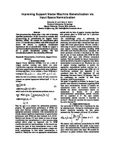
4.1.2 Separating instances into rings In this step we compute the angles of the projected instances in F with the central instance, φ(xc ), using K. The angles are stored in an array, which is then sorted. Here we have a choice of the number of instances that need to be included in a ring. The number of instances per ring can be based on the size of the L2 cache on the system to minimize cache misses. As we shall see later, only the instances in the same ring are processed together. Figure 1: Approximate Central Instance and Rings. Hence, at any given time during the processing of queries, we need only the amount of storage utilized 2. Separating the instances into rings based on their by the instances in one ring. angular distances from the central instance φ(xc ), Figure 1 shows the division of instances into differ3. Constructing a local indexing structure (intra-ring ent rings. To divide the instances into rings, we equally indexer) for each ring, and divide the sorted list. That is, if the number of instances 4. Creating an inter-ring index. per ring is g, then the first g elements in the sorted array are grouped together, and so on. This step requires 4.1.1 Finding the central instance As shown in O(n log n) time, and O(n) space. Figure 1, we attempt to find an approximate center φ(xc ) after the implicit projection of the instances to 4.1.3 Constructing intra-ring index For each the feature space F by kernel function K. The cosine ring, KDX constructs a local index. We construct for of the angle between a pair of instances is given by the each ring a g × g square matrix, where the ith row of the value of the kernel function K with the two instances matrix contains the angles between the ith instance and as input (see Equation 3.2). the other g − 1 instances. Next, we sort each row such that the instances are arranged according to decreasing Lemma 4.1. The closest approximation of the central order of similarity (or increasing order of distance) with instance is the projection of the instance xc whose sum the instance associated with the row. of distances from the other instances is the smallest. This step requires O(g 2 ) storage and O(g 2 d) + Proof. The point in F whose coordinates are the aver- O(g 2 log g) computational time for each ring. age of the coordinates of the projected instances in the dataset is at the center of the distribution of instances 4.1.4 Creating inter-ring index Finally, we conφ(xi ), i = 1 . . . n. Choosing the instance which mini- struct the inter-ring index, which is the closest instance mizes the variance gives us the closest approximation from the adjoining ring for each instance. This step reto the true center since it is closest to the point with quires O(n) storage and O(ng) time. All the steps above average coordinates in F. are essentially preprocessing of the data which needs to X be done only once for the dataset. 2 (φ(x ) − φ(x )) x = argmin c

i

xj

j

i

= argminxj

X

(φ(xi ) · φ(xi ) + φ(xj ) · φ(xj )

i

− 2φ(xi ) · φ(xj )) = argminxj

X

(2 − 2K(xi , xj )).

i

Given n instances in the dataset, each with d features, finding the central instance in the projected space takes O(n2 d) time. However, since we are only interested in the approximate central instance, this cost can be easily lowered via a sampling method. This step can be achieved with O(1) storage because at any point we need to store just the current known minimum, and the accumulated value of the sum of the angles of the rest of the instances with the current instance being evaluated.

4.2 KDX-top k In this section, we describe how KDX finds top-k instances relevant to a query (Definition 4.1) by just examining a fraction of the dataset. Details of the number of instances evaluated are presented in Section 5. Let us revisit Definition 4.1 for top-k relevant queries. The most relevant instances to a query, represented by a hyperplane trained by SVMs, are the ones farthest from the hyperplane on the positive side. Without an indexer, finding the farthest instances involves computing the distances of all the instances in the dataset from the hyperplane, and then selecting the k instances with greatest distances. This linear-scan approach is clearly costly when the dataset is large. Further, the number of dimensions associated with each data instance has a multiplicative effect on this cost.

KDX performs inter-ring and intra-ring pruning to find the approximate set of top-k instances by: 1. Shifting the hyperplane to the origin parallel to itself, and then computing θc , the angular distance between the normal to the hyperplane and the central instance φ(xc ). 2. Identifying the ring with the farthest coordinate from the hyperplane, and selecting a starting instance φ(x) in that ring. 3. Computing the angular separation between φ(x) and the farthest coordinate in the ring from the hyperplane, denoted as φ(x∗ ). 4. Iteratively, replacing φ(x) with a closer instance to φ(x∗ ) and updating the top-k list, until no “better” φ(x) in the ring can be found. 5. Identifying a good starting instance φ(x) for the next ring, followed by repeating steps 3 to 5, until the termination criterion is satisfied. KDX achieves speedup over the naive linear scan method in two ways. First, KDX does not examine all rings for a query. KDX terminates its search for top-k when the constituents of the top-k set do not change over the evaluation of multiple rings, or the query time expires. Second, in the fourth step, KDX examines only a small fraction of the instances in a ring. The remainder of this section details these steps, explaining how KDX effectively approximates the top-k result for achieving significant speedup. The formal algorithm is presented in Figure 8.

normal of the hyperplane2 can be written as Pm i αi yi φ(xl,i ) . (4.4) w = qP m i,j αi αj yi yj φ(xl,i ) · φ(xl,j ) The angular distance between the central instance and w is essentially cos−1 (w · φ(xc )). 4.2.2 Identifying the starting ring The most logical ring from which to start looking for the farthest instance is the one containing the coordinate on the hypersphere farthest from the hyperplane. Let φ(x¦ ) denote this farthest coordinate. Note that there may not exist a data instance at φ(x¦ ). However, finding an instance close to the farthest coordinate can help us find the farthest instance with high probability. The following lemma shows how we can identify the ring containing the farthest coordinate from the hyperplane. Lemma 4.2. The point, φ(x¦ ), on the surface of the hypersphere, farthest from the hyperplane, is at the intersection of the hypersphere and the normal to the hyperplane passing through the origin. The proof follows from the fact that all the instances are constrained to lie on the surface of a hypersphere and the distance from the hyperplane decreases as we move away from the point of intersection of the normal with the hypersphere because of the curvature. We do not need to explicitly compute the farthest coordinate, since we are only interested in the ring where it resides. To find the ring, we rely on the angular separation of φ(x¦ ) from φ(xc ), which is the θc obtained in the previous section. We use Figure 2 to illustrate. The figure shows that φ(x¦ ) is at the intersection of the hypersphere and the normal to the hyperplane with θc angular separation from φ(xc ). Given xc and the normal of the hyperplane, we can compute θc to locate the ring containing the farthest coordinate on the hypersphere from the hyperplane. The rings were formed from the sorted array of instances based on their angular separation from the central instance. Therefore, the first instance picked for every ring serves as a delimiter for that ring. To identify the ring, we therefore need to look only at these delimiters.

4.2.1 Computing θc Parameter θc is important for KDX to identify the ring containing the farthest coordinate from the hyperplane. To compute θc , we first shift the hyperplane to pass through the origin in the feature space. The SVM training phase learns the distance of the hyperplane from the origin in terms of variables b and w [19]. The distance of the hyperplane from the origin is given by −b/kwk. We shift the hyperplane to pass through the origin without changing its orientation by setting b = 0. This shift does not affect the set of instances farthest from the hyperplane because it has the same effect as adding a constant value to all distances. Next, we compute the angular distance θc of the central instance φ(xc ) from the normal to the hyperplane. Given training instances xl,1 . . . xl,m and their la- 4.2.3 Intra-ring pruning Our goal is to find the farthest instances in the ring bels y1 . . . ym , SVMs solve for weights αi for xl,i . The from the hyperplane. In this section, we present our pruning algorithm, which aims to reduce the number of instances examined to find a list of approximate farthest 2 Training instances with zero weights are not support vectors and do not affect the computation of the normal.

instances. In Section 5 we show that our pruning algorithm achieves high-quality top-k results, just by examining a small fraction of instances. If the ring is the first one being evaluated, KDX randomly chooses an instance φ(x) in the ring as the anchor instance. (In Section 4.2.4 we show that if the ring is not the first to be inspected, we can take advantage of the inter-ring index to find a good φ(x).) Let φ(x∗ ) be the farthest point from the hyperplane in the ring. We would like to find instances in the ring closest to φ(x∗ ). Our goal is to find these instances by inspecting as few instances in the ring as possible. Let us use a couple of figures to illustrate how this intra-ring pruning algorithm works. First, the circle in Figure 3 depicts the hyperdisc of the current ring. Please note that the hyperdisc can be inclined at an angle to the hyperplane as shown in Figure 4. Back to Figure 3. We would like to compute the distance s between φ(x) and φ(x∗ ). Since both φ(x) and φ(x∗ ) lie on the surface of a unit hypersphere, the angular separation between them can be obtained once s is known. Figure 3 shows that we need to determine h and v in order to use the Pythagorus theorem to obtain s. Determination of h and v, in turn, requires the knowledge of distances d1 and d2 . Distance d1 denotes the distance from the center of the hyperdisc to the hyperplane, along the hyperdisc, and d2 the distance of φ(x) to the hyperplane, along the hyperdisc. It is noteworthy that both these distances are measured along the surface of the hyperdisc as shown for d2 in Figure 4. We discuss in detail how we derive s in the online version of the paper at http://www.cs.ucsb.edu/˜panda/sdm complete.pdf. To focus our presentation on the pruning algorithm, we assume that we have had s computed. Given φ(x) and s, KDX at each step tries to find an instance farther than φ(x) from the hyperplane and closer to φ(x∗ ). Such an instance would lie between φ(x∗ ) and φ(x), or between φ(x∗ ) and point C, as depicted in Figure 5. Once we find a “better” instance than φ(x), we replace φ(x) with the new instance, and search for yet another farther instance. Notice that as we find a farther φ(x) from the hyperplane, the search range between φ(x) and C is reduced. This pruning algorithm eventually converges when no instances reside in the search range. When the pruning algorithm converges, there is a high probability that we have found a point φ(x) in the ring that is the farthest from the hyperplane. To understand the computational savings of this intra-ring pruning algorithm, let us move down to the next level of details. We use the example in Figure 6 to explain the pruning process. Starting at φ(x), we

ARC P’Q’

φ (x )

3 φ (x 1)

*

φ (x*)

P

φ (x ) 2

φ (x) φ (x4) φ (x5) φ (x 6)

φ (x 8) Q

φ (x ) 7

HYPERPLANE

Figure 6: Arrangement of instances seek to find an instance as close to φ(x∗ ) as possible. The intra-ring index (Section 4.1.3) of φ(x) contains an ordered list of instances based on their distances from φ(x). Let τ denote the angular separation between φ(x) and φ(x∗ ). To find an instance close to φ(x∗ ), we search this list for instances with an angular separation of about τ from φ(x). For the example in Figure 6 the neighboring points of φ(x) appear in the order φ(x3 ), φ(x1 ), φ(x4 ), φ(x5 ), φ(x2 ), φ(x6 ), φ(x7 ), and φ(x8 ) in the sorted list of φ(x). First, we need only examine the instances lying within the arc PQ in the figure, since an instance outside this arc cannot be closer to φ(x∗ ) than φ(x) itself. This step allows us to prune instances φ(x8 ) and φ(x7 ). Next, we would like to re-sort the instances remaining on the list of φ(x) based on their likelihood of being close to φ(x∗ ). To quantify this likelihood for instance φ(xi ), we compute how close the angular distance between φ(xi ) and φ(x) is to the angular distance between φ(x∗ ) and φ(x) (which is τ ). The list does not need to be explicitly constructed since we have sorted and stored the distances between φ(xi ) and φ(x) in the intra-ring index. Once we find the instance closest to φ(x∗ ) in the index, the rest of the instances on the re-sorted list can be obtained by looking up the adjacent instances of the closest instance in the intra-ring index. In our example, this re-sorted list is φ(x4 ), φ(x5 ), φ(x1 ), φ(x3 ), φ(x2 ) and φ(x6 ). It may be surprising that φ(x5 ) and φ(x4 ) appear before φ(x1 ) on the re-sorted list. The reason is that we know only the angular distance between two instances, not their physical order on the ring. Fortunately, pruning out φ(x5 ) and φ(x4 ) from the list is simple— we need only remove instances that are closer to the hyperplane than φ(x). In this case, φ(x5 ) and φ(x4 ) are closer to the hyperplane than φ(x). After removing

RING OF INTEREST

θ

s

φ((XC )

s

W

φ (x )

φ (x*)

φ (x)

C

v

φ (x) d2

r

d

φ (x)

φ (x*) C

RING

ψ

h RING

d 2

HYPERPLANE

d1

RING

Figure 4: Distance of φ(x) from inter- HYPERPLANE section of hyperplane and disc Figure 3: Finding s Figure 5: Stopping Figure 2: Start ring condition them from the re-sorted list, we harvest φ(x1 ) as the next instance for evaluation. Note that although φ(x1 ) is chosen in this cycle, the farthest instance from the φ (x1) hyperplane in the example is actually φ(x3 ). Next we φ (x) φ (x) use φ(x1 ) as the anchor instance for the next pruning φ (x ) iteration. 4 φ (x ) In the second pruning iteration, arc P’Q’ (obtained 3 using the ring associated with φ(x1 )) is the region that would be examined, anchored by φ(x1 ). In this step HYPERPLANE HYPERPLANE we use the re-sorted list of φ(x1 ) as well as that of its predecessor, φ(x), to choose the next anchor instance (a) agreed upon by both anchors. We pick the first instance (b) that is common in the re-sorted lists of all the anchors. Figure 7: Errors In the example, φ(x1 ) and φ(x) agree upon selecting φ(x3 ) as the next “better” instance. The algorithm tances with φ(x) are less than the value determined by converges at this point, since we do not have any more the width of the ring. Our method chooses the closest instances to examine. At the convergence point, we k neighbors of the best instance found in the ring and have obtained three anchor instances: φ(x), φ(x1 ), and updates the current set of top-k instances if necessary. φ(x3 ). This can induce errors when the top instances in the We make the following important observations on ring are located as in Figure 7(b). Here, if φ(x) is found KDX’s intra-ring pruning algorithm: to be the farthest instance in the ring, the choice of • At the end of the first iteration, we have indeed found top-k closest instances of φ(x) would prefer φ(x3 ) over the closest instance to φ(x∗ ) associated with φ(x). φ(x4 ). However, in practice, we see that the deviation Why do we look for the next anchor instance? Care- from the best possible distance values is relatively small. fully examining Figure 6, we can see that instance This means that although the top-k instances selected φ(x3 ), though farther than φ(x1 ) from φ(x∗ ), is ac- by KDX may not be exactly the same as the true set of k tually farther from the hyperplane than φ(x1 ). When farthest instances, their distances from the hyperplane the dimension of the hypersphere is high and the ring are very close to those of the farthest instances. has finite width, we can find instances farther from the hyperplane in many dimensions on the ring’s surface. 4.2.4 Finding starting instance in adjacent ring Having converged on a suitable instance (the approxi• In the case of a circle (2D ring with zero width) mate farthest instance) in a ring, we next use the interwe can argue about the optimality of the instance ring index to give us a good starting instance for the chosen by looking at the re-sorted list of the current next ring. The inter-ring index for an instance contains anchor alone, but the ring in our case is in very high the closest instance from the adjacent ring(s). Once we dimensional space and of non-zero width. Therefore, obtain the anchor instance, φ(x), for the new ring, we we use information available from any available rerepeat the intra-ring pruning algorithm in Section 4.2.3. sorted lists of prior anchors in the same ring to validate The algorithm terminates when the top-k list is not imthe choice of the next instance. proved after inspecting multiple rings. The algorithm Consider the ring shown in Figure 7(a). Suppose can also terminate when the wall-clock time allowed to the next instance chosen was φ(x), based on the stop- run the top-k query expires. ping criteria designed by us, it is possible for us to stop at φ(x). This is because φ(x1 ) lies outside the arc of 4.3 KDX-insertion and deletion interest of φ(x). The situation can be alleviated someInsertion into the indexing structure requires the idenwhat by considering the instances whose angular disHYPERPLANE

HYPERPLANE

Algorithm 4.1. KDX-top k Input: Support vectors zi Procedure Adjacent(R) Dataset instances xi 1: static direction = 0 Intra-ring index Arr 1: 2: static num1 = 1, num2 = 1 Inter-ring index inter ring 3: if direction = 0 and R + num1 < n/g then Output: Top-k set top k 4: R0 = R + num1 2: counter = 0 5: num1 = num1 + 1 3: condition = False 6: else if R − num2 ≥ 0 then 4: top k = {} 7: R0 = R − num2 5: θc = Find θc (zi , xc ) 8: num2 = num2 + 1 6: R = Find ring of interest(θc , ring) 9: end if 7: ψ = Find ψ(θc ) 10: direction = 1 − direction 8: R0 = R 11: return R0 9: x = random instance in R 10: while counter < n/g and condition = False do Procedure Find h v(d1 , d2 , x, xc , w) 11: Converged = False Section 4.2.3 12: S = {} 1: r = sin(cos−1 (φ(x) · φ(xc )) 13: while !Converged do 2: if d1 × d2 ≥ 0 and d1 ≥ 0 then 14: (d1 , d2 ) = Find distances(x, w, ψ) 3: temp = d2 − d1 15: (h, v) = Find h v(d1 , d2 , x, xc , w) 4: v = abs(temp − r) 16: (τ, ξ) = Find τ ξ(h, v) 0 17: index = Bin search( Arr[R ][ inverted index[x]], τ ) 5: else if d1 ≥ 0 then 0 6: temp = d1 − d2 18: if ring[R ][index] == x then 7: v = r + temp 19: Converged = True 8: else 20: else 0 9: temp = d2 − d1 21: Sx = Arrangement(x,τ ,ξ,R ) v = r − temp 22: xn = ∩S // Intersection chooses unevaluated in- 10: 11: end p if stance only 12: h = r2 − temp2 23: x = xn 24: end if Procedure Find τ ξ(h, v) 25: end while Section 4.2.3 26: condition = Ring termination condition(top k, x) √ 27: x = inter ring(x) 1: s = h2 + v 2 0 2 28: R = Adjacent(R) ) 2: τ = cos−1 ( 2−s 2 29: counter = counter + 1 2 −1 2−(2h) ) 3: ξ = cos ( 30: end while 2 Procedure Arrangement(x, τ, ξ, R0 ) Procedure Find θc (zi , xc ) Section 4.2.1 1: zi ← Support vector i P

2: w =

3: θc =

1: 2: 3: 4: 5:

nsv αi yi φ(zi ) i qPn sv α α y y φ(z )·φ(z ) i j i j i j i,j cos−1 (w · φ(xc ))

Procedure Find ring of interest(θc , ring) Section 4.2.2 1: for i = 1 to num rings do 2: temp array[i] = cos−1 (K(ring[i][0], xc )) 3: end for 4: R = Bin Search( temp array, θc ) Procedure Find ψ(θc )

1: if θc > π/2 then 2: ψ = π − θc 3: else 4: ψ = θc 5: end if Procedure Find distances(x, w, ψ)

1: 2: 3: 4:

d = w · φ(x) d2 = d/sin(ψ) p = φ(x) · φ(xc ) d1 = p/tan(ψ)

6: 7: 8: 9: 10: 11: 12: 13: 14:

temp S = {} index1 = Bin search( Arr[R0 ][inverted index[x]], τ ) index2 = Bin search( Arr[R0 ][inverted index[x]], ξ ) counter = 0 while index1+counter < index2 or index1−counter > 0 do if index1 + counter < index2 then temp S = temp S ∪ Arr[R0 ][x][index1 + counter] end if if index1 − counter > 0 then temp S = temp S ∪ Arr[R0 ][x][index1 − counter] end if counter = counter + 1 end while return temp S

Procedure Ring termination condition(top k, x)

1: 2: 3: 4: 5: 6: 7: 8: 9: 10: 11: 12: 13: 14:

static f lag = 0 ring top k = k nearest neighbors of φ(x) for i = 1 to k do Merge ring top k and top k if top k modified then f lag = 0 else f lag = f lag + 1 end if end for if f lag == num unproductive rings then return True end if return False

Figure 8: Algorithm for top-k retrieval tification of the ring to which the new instance belongs and an update of the indexing structure of the ring. Identification of the ring requires O(log(|G|)) time, |G| being the number of rings. Updating the index struc-

ture within the selected ring requires O(g) time, g being the number of instances in the ring. Insertion of instances does change the central instance. We are interested in an approximate central instance, which can

roughly ensure that the instances are evenly distributed in each ring. Addition of fresh instances does not disturb this situation, and hence the re-computation of the central instance is not mandatory. However, when the number of instances added is high compared to the existing dataset size, the possibility of a skewed distribution of the instances in the rings is higher. In such a case a re-computation of the central instance and the index would be beneficial. If we assume that the current set of instances in the dataset is representative of the distribution of instances, the approximate central instance represents a viable choice even after the insertion of new instances into the database. We discuss the details in the online version of the paper at http://www.cs.ucsb.edu/˜panda/sdm complete.pdf. 4.4 KDX-changing kernel parameters In this section we discuss methods that allow us to perform indexing using the existing indexing structure when the kernel parameters can change. The form of the kernel function is assumed to remain the same. That is, if we had built the index using the Gaussian kernel, we would continue using the Gaussian kernel, but the parameter σ to the kernel would be allowed to change. Suppose we wish to look at the ordering of the angles made by instances with a fixed instance say xf . We are interested in the values taken on by the function K(xi , xf ), where xi is any instance in the dataset. Consider the Gaussian kernel. The values of kx −x k2 interest are given by K(xi , xf ) = exp(− i2σ2f ). Since the exponential function is monotonic in nature, the ordering of instances based on their angular separation from xf does not change with a change in parameter σ. The same follows for the Laplacian kernel. The polynomial kernel which has the form (1 + xi · xf )p is also monotonic in nature if p ≥ 1 and xi · xf ≥ 0, ∀xi . Replacing xf by the central instance, we see that the ordering of instances based on their angular separation with the central instance does not change with change in the kernel parameter. Effectively, this means that the grouping of instances into rings, given a particular form of the kernel function, is invariant with change in the kernel parameter. Further, each row of the intra ring index is essentially the ordering of the instances in the ring based on their angular separation with the instance associated with that row in the ring. Again, these orderings are unaffected by changes in the value of the kernel parameter. The functioning of the indexing approach outlined before locates a given angle in the sorted array of angles using binary search. Now, after changing the kernel parameter, we do not have the values of the angles which were used to construct the array. But, since the ordering

is unchanged, we can compute the values on the fly when we access an instance in the course of the binary search operation. Finally, we turn our attention to the inter-group index. Since this index stores the closest instance from the adjacent group, the monotonic nature of the kernel functions implies that this index is completely unchanged. Thus, the old indexing structure can be used unchanged by computing only the required values when necessary. Since binary search in an array of size g takes O(log g) time, therefore the extra computations that need to be performed are of the order O(log g) for each binary search operation. 5

Experiments

Our experiments were designed to evaluate the effectiveness of KDX using a variety of datasets, both small and large. We wanted to answer the following questions: • Are the top-k instances chosen by KDX of good quality? • Quantitatively, how good are the results in terms of their distances from the hyperplane? • How effective is KDX in choosing only a subset of the data to arrive at the results? • How does the change in parameters (number of instances per ring and kernel parameter) affect the performance of KDX? Our experiments were carried out on four UCI datasets [4], a 21k-image dataset, and a 300k-image dataset (obtained from Corbis). The four UCI datasets were selected because of their relatively large sizes; the two selected image-datasets have been used in several research prototypes [7]. The details of the datasets are presented in Table 1. In our experiments on topk retrieval we obtained results for k = 10, 20 and 50 for the Corbis dataset, and k = 20 for the rest of smaller datasets. The experiments were carried out with the Gaussian kernel. UCI Datasets We chose four UCI datasets— namely, Seg, Wine, Ecoli and Yeast. Seg: The segmentation dataset was processed as a binary-class dataset by choosing its first class as the target class, and all other classes as the non-target classes. We then performed a top-k query on the first class. Wine: The wine recognition dataset comes from the chemical analysis of wines grown in the same region of Italy but derived from three different cultivators. Each instance has 13 continuous features associated with it. The dataset has 180 instances. We performed three topk queries on their three classes.

Dataset Seg Wine Yeast Ecoli 21-k Image Corbis

# Classes # Training # Testing 1 109 103 3 93 87 10 747 737 8 165 171 116 4,321 16,983 1,173 1,789 312,712 Table 1: Dataset description

Yeast: The yeast dataset is composed of predicted attributes of protein localization sites. The dataset contains 1, 484 instances with eight predictive attributes and one name attribute. Only the predictive attributes were used for our experiments. This dataset has ten classes, but since the first three classes constitute nearly 77% of the data, we used only these three. Ecoli: This dataset also contains data about the localization pattern of proteins. It has 336 instances, each with seven predictive attributes and one name attribute. It has eight classes out of which the first three represent roughly 80% of the data and hence were used for our experiments. 21-k Image dataset The image dataset was collected from the Corel Image CDs. Corel images have been widely used by the computer vision and imageprocessing communities. This dataset contains 21-K representative images from 116 categories. Each image is represented by a vector of 144 features including color, texture and shape features [7]. Corbis dataset Corbis is a leading visual solutions provider (http://pro.corbis.com/). The Corbis dataset consists of over 300, 000 images, each with 144 features. It includes content from museums, photographers, filmmakers, and cultural institutions. We selected a subset of its more than one thousand concepts. The number of training and test instances vary slightly with the different classes in the same dataset because of differences in the number of positive samples in each class. The samples were randomly picked from both positive and negative classes. In the case of the smaller datasets (Seg, Wine, Yeast and Ecoli), the percentages of positive and negative samples picked were equal. We chose 50% of the entire dataset was chosen as training data. For the larger datasets (21k image and the Corbis) the percentage of positive samples picked was higher (50%) than the percentage of negative samples chosen. This was done to ensure that the large volume of negative samples does not affect the SVM training algorithm, which is sensitive to imbalances in the sizes of the training and testing datasets. The details of the separation of the datasets are presented in Table 1.

5.1 Qualitative evaluation Given a query, KDX performs a relevance search to return the k farthest instances from the query hyperplane. To measure the quality of the results, we first establish a benchmark by scanning the entire dataset to find the top-k instances for each query: this constitutes the “golden” set. The metric we use to measure the query result is recall. In other words, we are interested in the percentage of top-k golden results retrieved by KDX. Results for the qualitative evaluation are presented in the second column of Table 2. The results are averaged over three classes for all the datasets except for Seg. The average recall values for all datasets are above 80%. For the Corbis dataset, which has the largest number of instances, we have an average recall of 90% with less than 4% of data evaluated. (We report recall vs. fraction of data evaluated in Section 5.3.) The recall values are reasonably high for all the datasets. 5.2 Evaluation of discrepancy This quantitative evaluation involved finding the discrepancy between the average distance to the hyperplane from the top-k instances found by KDX, and the average distance to the hyperplane from the top-k instances in the “golden” set. To obtain a percentage, we divide the average discrepancy by the difference of the distances of the most positive and least positive instances in the dataset. The results showing the percentage of average discrepancy for all the datasets are presented in the third column of Table 2. The low values of the percentage of average discrepancy indicate that even if the retrieved instances may not exactly match the golden set of top-k instances, they are comparable in their distances from the hyperplane. None of the datasets has more than 0.3% average discrepancy with the values being very low for the large datasets. 5.3 Percentage of data evaluated This evaluation aimed to find the percentage of data evaluated before we obtained the best results using the indexing strategy. In other words, we were interested in finding approximately how quickly KDX converged on its set of best results. The results are reported in the fourth column of Table 2. These values are mostly very low (lower than 10%) except in the case of the smaller datasets where, because of the small size of the dataset, the percentage of evaluated samples, even with a small number of samples being evaluated, tends to be high. For the large datasets, we find that the results are impressive with less than 4% of the data being evaluated to reach 90% recall. Figure 10 gives a detailed report of the percentage of average discrepancy, percentage of evaluated samples,

% Average discrepancy (σ2 =30) (σ2 =40) (σ2 =60) (σ2 =70)

5 4

4

3

3

2

2

20 15

15

10

10

100

100

90

90

80

80

70

70

60

60

50

50

40

40

30 5

5

1

1

% Evaluated samples (σ2 =30) (σ2 =40) (σ2 =60) (σ2 =70)

20 % of data evaluated

% discrepancy

5

25

25

% Recall

6

6

% Recall (σ =30) (σ2 =40) (σ2 =60) (σ2 =70)

20 10

0 0

50

100

150

200

250

300

0 350

0 0

50

Number of rings examined

100

150

200

250

300

0 350

30

2

0 0

50

Number of rings examined

100

150

200

250

300

20 10 0 350

Number of rings examined

Figure 9: Corbis dataset: variation with change in σ 2 from 30 to 70 % Average discrepancy (750 points) (1000 points) (1250 points) (1500 points)

% discrepancy

5

5 4

4 3

3

2

2

1

1

0

0 0

0.2

0.4

0.6

0.8

Fraction of rings examined

1

18

1.2

% Evaluated samples (750 points) (1000 points) (1250 points) (1500 points)

16

6 % of data evaluated

6

14 12

18

100

100

16

90

90

14

80

80

70

70

60

60

50

50

40

40

12 % Recall

7

7

10

10

8

8

6

6

4

4

20

2

2

10

0

0

0

0

0.2

0.4

0.6

0.8

Fraction of rings examined

1

1.2

30

30

% Recall (750 points) (1000 points) (1250 points) (1500 points)

20 10 0

0

0.2

0.4

0.6

0.8

1

1.2

Fraction of rings examined

Figure 10: Corbis dataset: variation with change in number of points per ring from 750 to 1500 (σ 2 = 50) and the change in recall as the number of rings increases. In each of the graphs, the x-axis depicts the fraction of the total number of rings processed, and the yaxis depicts the different quantities of interest. The recall (presented in the right-most graph in Figure 10) reaches a peak early in the evaluation with only a few instances being explicitly evaluated (presented in the middle graph). The discrepancy falls to its lowest level with roughly 4% of the data being evaluated (presented in the left-most graph). 5.4 Changes in parameters This set of experiments focused on two different parameters. In the first set of experiments, we were interested in evaluating the performance of the indexing strategy when the kernel parameter (in this case σ of the Gaussian kernel) was changed after the index had been constructed. The second set of experiments evaluated the performance of the indexing strategy when the number of instances per ring was varied. Figure 9 shows the results obtained by varying kernel parameter σ 2 between 30 and 70 for the Corbis dataset. Here the x-axis depicts the number of rings examined and the y-axis the quantities of interest (average discrepancy, percentage of data evaluated, and recall). As σ decreases, the angular separation between instances increases, and so does the width of each ring. This affects recall since with wider rings KDX

can miss instances as shown in Figure 7(a). However, the extremely low discrepancy values indicate the high quality of the selected instances. Figure 10 shows the results of changing the number of points in the rings for the Corbis dataset from 750 points to 1, 500. Though recall generally improves when the number of instances per ring decreases, the percentage of evaluated instances increases. The above results indicate that changes in kernel parameters and number of points in the ring within reasonable limits do not significantly affect KDX’s performance. We also experimented with different k values for the Corbis dataset. The results of k = 10 and k = 50 are reported in Table 3. When k is small, the recall tends to suffer slightly; when k is large, the recall can approximate 100%. In both cases, the distance discrepancy remains very small (less than 0.1%). Although KDX may occasionally miss a small fraction of the “golden” top-k instances, the quality of the top-k found is very good. 6 Conclusions We have presented KDX, a novel indexing strategy for speeding up top-k queries for SVMs. Evaluations on a wide variety of datasets were carried out to confirm the effectiveness of KDX in converging on relevant instances quickly. As future work we would like to pursue the goal

Dataset

% Recall

% Discrepancy

% Evaluated till recall Seg 100 0 7.84314 Wine 93.3 0.27225 22.4806 Yeast 80.0 0.06603 3.547 Ecoli 100 0 17.2647 21K 85.0 0.0272883 2.8559 Corbis 90.0 0.03607813 2.94255 Table 2: Qualitative and quantitative comparison Dataset

Class

Recall

% Discrepancy

Corbis (k = 10)

0 1 2 0 1 2

0.8 1 0.7 0.98 0.96 0.9

0.05241 0 0.119966 0.000324724 0.00851683 0.036358

Corbis (k = 50)

% Evaluated till recall 3.7729 1.82111 2.91755 3.83965 1.84253 3.06362

Table 3: Results with varying k of further lowering the number of instances to be evaluated. We would also like to develop bounds on the number of instances that KDX evaluates. Another objective would be to lower the size of the index structure used by KDX. Currently, the index structure takes up O(n g) space (g being the number of instances in each ring). Although the dataset itself takes up O(n d) space (d being the dimensionality of each feature vector), the size of the index structure can quickly become very large. We would like to explore avenues restricting the size of the index.

[8]

[9]

[10]

[11]

[12]

[13]

[14]

[15]

References [1] Charu C. Aggarwal and Philip S. Yu. Outlier detection for high dimensional data. In SIGMOD Conference, 2001. [2] N. Beckmann, H. Kriegel, R. Schneider, and B. Seeger. The R∗ tree: An efficient and robust access method for points and rectangles. In ACM SIGMOD Int. Conf. on Management of Data, pages 322–331, 1990. [3] S. Berchtold, D. Keim, and H.P. Kriegel. The X-tree: An index structure for high-dimensional data. In 22nd Conference on Very Large Databases, Bombay, India, pages 28–39, 1996. [4] C.L. Blake and C.J. Merz. UCI repository of machine learning databases, 1998. [5] M. Brown, W. Grundy, D. Lin, N. Christianini, C. Sugnet, M. Jr, and D. Haussler. Support vector machine classification of microarray gene expression data. 1999. [6] Christopher J.C. Burges. Geometry and invariance in kernel based methods. In Alex J. Smola Bernhard Sch¨ olkopf, Chris Burges, editor, Advances in Kernel Methods. MIT Press Cambridge, MA, 1998. [7] E. Chang, K. Goh, G. Sychay, and G. Wu. Contentbased soft annotation for multimodal image retrieval

[16]

[17]

[18]

[19] [20]

using bayes point machines. IEEE Trans. on Circuits and Systems for Video Technology Special Issue on Conceptual and Dynamical Aspects of Multimedia Content Description, 13(1):26–38, 2003. P. Ciaccia, M. Patella, and P. Zezula. M-tree: An efficient access method for similarity search in metric spaces. Proc. 23rd Int. Conf. on Very Large Databases, pages 426–435, 1997. Aristides Gionis, Piotr Indyk, and Rajeev Motwani. Similarity search in high dimensions via hashing. In The VLDB Journal, pages 518–529, 1999. Michael E. Houle and Jun Sakuma. Fast approximate similarity search in extremely high-dimensional d ata sets. In ICDE, 2004. Thorsten Joachims. Text categorization with support vector machines: learning with many relevant features. In Claire N´edellec and C´eline Rouveirol, editors, Proceedings of ECML-98, 10th European Conference on Machine Learning, number 1398, pages 137–142, Chemnitz, DE, 1998. Springer Verlag. Norio Katayama and Shin’ichi Satoh. The SR-tree: an index structure for high-dimensional nearest neighbor queries. In ACM SIGMOD Int. Conf. on Management of Data, pages 369–380, 1997. D. A. Keim. Tutorial on high-dimensional index structures: Database support for next decades applications. In Proceedings of the ICDE, 2000. Hyunsoo Kim, Peg Howland, and Haesun Park. Dimension reduction in text classification using support vector machines. Journal of Machine Learning Research, to appear. Chen Li, Edward Chang, Hector Garcia-Molina, and Gio Wilderhold. Clindex: Approximate similarity queries in high-dimensional spaces. IEEE Transactions on Knowledge and Data Engineering (TKDE), 14(4), July 2002. King-Ip Lin, H. V. Jagadish, and Christos Faloutsos. The TV-tree: An index structure for highdimensional data. VLDB Journal: Very Large Data Bases, 3(4):517–542, 1994. Simon Tong and Edward Chang. Support vector machine active learning for image retrieval. ACM International Conference on Multimedia, pages 107– 118, 2001. Simon Tong and Daphne Koller. Support vector machine active learning with applications to text classification. In Pat Langley, editor, Proceedings of ICML00, 17th International Conference on Machine Learning, pages 999–1006, Stanford, US, 2000. Morgan Kaufmann Publishers, San Francisco, US. V. Vapnik. The Nature of Statistical Learning Theory. Springer Verlag, 1995. Roger Weber, Hans-J¨ org Schek, and Stephen Blott. A quantitative analysis and performance study for similarity-search methods in high-dimensional spaces. In Proc. 24th Int. Conf. Very Large Data Bases, VLDB, pages 194–205, 24–27 1998.

A

Center instance lemma

Lemma A.1. The closest approximation of the central instance is the instance xc whose sum of distances from the other instances is the smallest. Proof. The point in F whose coordinates are the average of the coordinates of the projected instances in the dataset is at the center of the distribution of instances φ(xi ), i = 1 . . . n. Choosing the instance which minimizes the variance gives us the closest approximation to the true center since it is closest to the point with average coordinates in F. X (φ(xi ) − φ(xj ))2 xc = argminxj

φ (XC)

W

ψ θ

ψ

φ (XC) θ

W

C

C

Figure 12: Finding the angle of inclination φ

(X)

φ

r

(X ) C

p

i

= argminxj

X

(φ(xi ) · φ(xi ) + φ(xj ) · φ(xj )

i

− 2φ(xi ) · φ(xj )) = argminxj

X

(2 − 2K(xi , xj )).

i

B Finding the values of d1 , d2 and ψ We now discuss the geometrical aspects of the proposed method and demonstrate how the various values (d1 , d2 and r) in Figure 3 are computed. Essentially the rings can be visualized as in Figure 2. Visualizing the situation from a direction parallel to the surface of the rings gives us Figure 3. Here we have shown the hyperplane passing through the origin but this is not necessary for our method since a hyperplane which does not pass through the origin can always be shifted parallel to itself to the origin without changing the instances which are farthest away from it in the positive half-space. The only situation where we would not be able to do this is when the hyperplane was such that all the instances were only in the negative half-space, but then such a hyperplane is useless. B.0.1 Computation of ψ Observing Figure 2 we note that the rings formed by each of the rings are inclined at the same angle to the hyperplane (and hence its normal) The angle of inclination can be found by computing the angular separation of the central instance with the normal. If the central instance makes an angle greater than π/2 with the normal and its angular separation from the normal is θc then the angle of inclination ψ is given by (2.5)

ψ = π − θc .

If the central instance makes an angle of less than π/2 with the normal to the hyperplane then the angle of inclination is given by (2.6)

ψ = θc .

Figure 13: Determination of the radius Both the situations are presented in Figure 12. B.0.2 Computation of distances d1 and d2 Once the angle of inclination has been determined we can find the distance of φ(x) from the intersection of the hyperplane with the surface of the ring. We know the distance of φ(x) from the hyperplane. In Figure 4 this is represented by d. Knowing d and the angle of inclination allows us to compute d2 . The radius of the ring, r in Figure 13 can be computed since we know the radius of the hypersphere (1) and the angle between φ(x) and φ(xc ). Similarly, we can determine p which is the distance of the center of the ring from the origin O. Once p has been determined the distance of the center from the intersection of the hyperplane and the disc (d1 ) can be directly computed since we know the angle of inclination of the disc to the hyperplane. Thus we have d1 = p/tan(ψ). B.1 KDX-insertion and deletion Insertion into the indexing structure requires the identification of the ring to which the new instance belongs and an update of the indexing structure of the ring. Identification of the ring requires O(log(|G|)) time, |G| being the number of rings. Updating the index structure within the selected ring requires O(g) time, g being the number of instances in the ring. Insertion of instances does change the central instance. We are interested in an approximate central instance, which can roughly ensure that the instances are evenly distributed in each ring. Addition of fresh instances does not disturb this situation and hence the re-computation of the central instance is not mandatory. However, when the number of instances added is high compared to the existing dataset size then the possibility of a skewed distribution of the instances

Create index Dataset instances xi Number of instances per ring g Output: Central instance xc Intra-ring index Arr Inter-ring index inter ring Ring entries ring

Algorithm A.1. Input:

1: 2: 3: 4: 5:

xc =Find central(xi ) ring = Separate instances(xi , xc , g) Arr = Create intra ring index(ring, g, xi ) inter ring = Create inter ring index(ring, xi , g)

Procedure Find central(xi )

1: n = Number of instances in dataset 2: min = inf 3: c /* Index of central instance */ 4: for i = 1 to n do 5: sum[i] = 0 6: for j = 1 to n do 7: sum[i] + = (2 − 2K(xi , xj )) 8: end for 9: if min > sum[i] then 10: min = sum[i] 11: c = i 12: end if 13: end for

Procedure Create intra ring index(ring, xi , g)

1: 2: 3: 4: 5: 6: 7: 8: 9:

g = Number of instances in each ring for i = 1 to n/g /*Cycle over all rings*/ do for j = 1 to g do for k = 1 to g do Arr[i][j][k] = K(xring[i][j] , xring[i][k] ) end for Sort( Arr[i][j] ) end for end for

Procedure Create inter ring index(ring, xi , g)

1: for i = 1 to n/g − 1 do 2: for j = 1 to g do 3: max = 0 4: for k = 1 to g do 1: for i = 1 to n do 5: if K(xring[i][j] , xring[i+1][k] ) > max then 2: anglec [i] = K(xi , xc ) 6: max = K(xring[i][j] , xring[i+1][k] ) 3: indexc [i] = i 4: end for 7: inter ring[ring[i][j]][0] = ring[i + 1][k] 5: Sort( anglec , indexc ) /* indexc stores the instance number after 8: end if sorting*/ 9: end for 6: r = 1 10: end for 7: for j = 1 to n do 11: for j = 1 to g do 8: if j%g == 0 then 12: max = 0 9: r = r+1 13: for k = 1 to g do 10: end if 14: if K(xring[i][j] , xring[i−1][k] ) > max then 11: ring[r][j%g + 1] = indexc [j] max = K(xring[i][j] , xring[i−1][k] ) 12: inverse index[indexc [j]] = j%g + 1 /*Stores the position in the 15: ring*/ 16: inter ring[ring[i][j]][1] = ring[i − 1][k] 13: end for 17: end if 18: end for 19: end for 20: end for Procedure Separate instances(xi , g, xc )

Figure 11: Algorithm for creating the index in the rings is higher. In such a case a re-computation of the central instance and the index would be beneficial. If we assume that the current set of instances in the dataset is representative of the distribution of instances, the approximate central instance represents a viable choice even after the insertion of new instances into the database. Visually, we explain the situation in Figure 14. The first ring shows instances before insertion. The same ring has been shown in the adjacent figure with a large number of instances added asymmetrically. After the new instances have been added into the index we resume computation using the old central instance. The search for the most suitable instance within the ring proceeds as before. The new ring with inserted instances can essentially be seen as an asymmetric ring. If the inserted instances are symmetrically distributed across the ring, there is no effect on the search for the best instance in the ring. In the case where the new instances are mostly added in a small region of the ring, the effect is only seen when the instance of interest lies approximately in that region. The effect is that of having a larger number of possible candidates in the ini-

x

x

x

x

x

x

x

x

x

x O x

x x

x x

x

x x

x x x x x x x x x x x x x x x x x

x

x O x x x

x

x x

Figure 14: Effect of inserting new instances tial step which are pruned out as we approach the best instance. The overall effect is that of slowing the rate of convergence by a few steps. It is important to note that this would happen in the case of any ring which has such uneven distribution of instances and cannot be attributed to the decision not to recompute the central instance, since even a recomputation of the central instance does not guarantee that the rings will not have an uneven distribution of instances. When the instance of interest does not lie in the region where most of the new instances lie, the new instances are pruned out at a very early stage thus not affecting the search for the

most suitable instance. When the inter ring index is queried for a good starting point the inserted instances in fact aid by allowing the inter ring index to choose with a finer granularity as compared to before. The computation of the central instance allows us to divide the instances in the dataset into rings so that at least some of the rings have an even distribution of instances. Finding a good starting point speeds up processing in the ring by by narrowing down the possible candidates. Essentially, the choice of instance using the inter ring index would not be as good as in the case of an even distribution but since we do not rely completely on the inter ring index for the selection of the best instance in a ring, this effect is at best minimal. Thus, the deletion of instances from a ring does not affect the indexing scheme radically. Deletion of instances involves removing the corresponding row and column from the associated index and takes O(g) time. This cost can be completely avoided if we maintain a record of the deleted items and avoid them when presenting results. Deleted instances which haven’t been removed are also useful when finding a good starting point in the next ring using the inter ring index. C

Cost analysis

In this section we discuss the costs associated with our indexing strategy in various scenarios. The scenarios we discuss are

we mean that the distance of the instance from the hyperplane was evaluated explicitly using the weighted support vectors. Thus, if there were n instances in the dataset and only m needed to be explicitly evaluated by the indexing scheme then the speedup would be of the order n/m. Let us consider the case when not all the instances and the associated index structures can be loaded into memory at the same time. Considering only the memory used by the instances without the indexing structure, let it be possible to load n instances out of a total of N instances into memory at the same time. If the number of features associated with each instance is d then the total memory available is given by n × d. Since each ring consumes g ×g +g ×d space, we can load n×d g×g+g×d rings into memory at a time. Let the number of rings be c. We have c = N/g. The number of disc accesses is given by c × (g × g + g × d) . n×d This can be simplified to N (g × g + g × d) g N = (1 + ) . n×g×d d n Thus, the total disc access time is given by g N TD (1 + ) . d n

If the fraction of instances that needed to be completely evaluated is F then the time required to evaluate these • The best ring has been identified and only a subset is given by of the rings are examined. TC (F × N × d × nsv ), • All the rings are examined.

• An alternative strategy is discussed wherein the where nsv is the number of support vectors and TC is the required arrays are computed as and when required. time required for a single floating point computation. This strategy is aimed at minimizing the memory The total time required is given by consumption. g N (3.7) TD (1 + ) + TC (F × N × d × nsv ). We discuss each of the scenarios in detail below. d n C.1 Case 1: All rings are examined Every ring in our indexing scheme maintains an intra ring index which is essentially a square array of size equal to the number of instances in the ring. Let the instances be equally divided into rings such that each instance contains g instances. The amount of memory consumed by each ring for its intra ring index is O(g 2 )‘ When all the instances as well as the intra ring indexes can be loaded into memory at the same time at load time, the indexing scheme does not suffer any delays because of disc accesses and the speedup observed depends solely on the number of instances which needed to be completely evaluated. By complete evaluation,

The time spent by the sequential algorithm in evaluating all the instances is given by N × d × nsv × TC . The number of disc accesses here is N/n and therefore, the total time taken is given by (3.8)

TD

N + TC × N × d × nsv . n

The speedup is given by (3.9)

TD N n + TC × N × d × nsv . g N TD (1 + d ) n + TC (F × N × d × nsv )

It is easy to see that because of the high cost of disc access (TD ) as compared to processing cost (TC ), it is impossible to beat the sequential scan when all the rings are examined. The only situation where it is possible to do so is when all the rings can be loaded into memory at the same time. Such a case is possible when distributed evaluation of queries takes place with the instances in the various rings being spread over multiple computers. This is usually the case for search engines attempting to address user queries quickly.

the ordering of instances with respect to the central instance, the instances belonging to any given ring is known. Having chosen a ring and an instance for evaluation, we need to find its angular separation from the rest of the instances in the ring. This can be accomplished in O(g d) time. Sorting the values obtained takes O(g log g) time. The rest of the steps are essentially the same. Thus we have negated the cost of the disc accesses since the number of disc accesses is essentially the same as the number of disc accesses in the case of the sequential access of instances. The computational cost associated is given by

C.2 Case 2: Subset of rings examined This brings us to the alternate strategies. The next strategy starts from the most suitable ring for the given query TC × F × N × (d × nsv + g × d + glogg). and examines only a subset of all the rings. Since we are starting from the ring which can possibly contain The computational cost associated with the sequenthe best instance, examination of a subset of the rings tial scan is given by would be enough in most cases to obtain a reasonably good approximate solution. Let the number of rings TC × N × d × nsv . that are examined be t then the number of disc accesses is given by Therefore, the speedup here is given by t × (g 2 + g × d) , d × nsv n×d F × (d × n sv + g × d + glogg) and the total time taken for this operation is given by TD

t × (g 2 + g × d) . n×d

The processing time is given by TC F tgdnsv Hence the speedup is given by TD N n + TC × N × d × nsv TD

t×(g 2 +g×d) n×d

+ TC × F × t × g × d × nsv

.

We can control the number of disc accesses by controlling the number of rings we examine. C.3 Case 3: Just in time computation The final strategy we outline is the just in time strategy. It is important to note that we only access part of the index that we have created in the preprocessing stage. The rest of the index which is not used consumes memory space without being useful. Since computation cost is much lesser than the cost of disc access we would like to minimize the number of disc accesses by minimizing the size of the index we store. Here, in addition to the instance vectors we only store the ordering of instances with respect to their angular distance from the central instance and the inter ring index. In other words, we wish to compute the intra ring index as and when required. Since we maintain