Uncertainty and the Great Recession∗ Benjamin Born, Sebastian Breuer, Steffen Elstner This version: June 7, 2017

Abstract Has heightened uncertainty been a major contributor to the Great Recession and the slow recovery in the U.S.? To answer this question, we identify exogenous changes in six uncertainty proxies and quantify their contributions to GDP growth and the unemployment rate. The answer is no. In total we find that increased macroeconomic and financial uncertainty can explain up to 10 percent of the drop in GDP at the height of the recession and up to 0.7 percentage points of the increased unemployment rates in 2009 through 2011. Our calculations further suggest that only a minor part of the rise in popular uncertainty measures during the Great Recession was driven by exogenous uncertainty shocks.

1

Introduction

How much has increased uncertainty contributed to the Great Recession and the ensuing weak recovery in the United States? This question has captivated economists, politicians, and the blogosphere alike, the popular argument being that uncertainty reduces firms’ hiring ∗

Born: University of Bonn, CEPR, and CESifo, email: [email protected]; Breuer: German Council of Economic Experts, email: [email protected]; Elstner: RWI Essen, email: [email protected]. We would like to thank the editor, two anonymous referees, Rüdiger Bachmann, Johannes Pfeifer, and participants at the 2015 World Congress of the Econometric Society, the 2015 EEA meeting, the 2015 Annual Meeting of the Royal Economic Society, the 2014 Annual Meeting of the Verein für Socialpolitik, and seminar audiences at IFO Institute Munich and Deutsche Bundesbank for helpful comments and suggestions.

1

and investment and consumers’ spending. However, while the literature on the effects of fluctuations in uncertainty on economic activity has rapidly expanded following the seminal paper by Bloom (2009),1 few papers have actually quantified the specific effects of uncertainty on U.S. GDP and unemployment in the aftermath of the financial crisis. In a “back-of-theenvelope” calculation, Bloom (2014) reckons that the rise in uncertainty in 2008 potentially accounted for a three percentage point loss in GDP in 2008 and 2009. Baker et al. (2016) find that the increase in policy uncertainty during the years 2006 to 2011 can be connected to a decline in industrial production of 1.1 percent.2 For the U.S. unemployment rate, Leduc and Liu (2016) find that uncertainty shocks account for a one percentage point increase during the crisis and recovery.3 We contribute to this literature by providing quantitative estimates of the pure uncertainty effects on the U.S. economy since 2008. To this end, we use structural vector autoregressions (SVAR) and identify monthly exogenous changes in a wide range of uncertainty proxies. We then compute historical decompositions to determine the effects of these identified uncertainty shocks on GDP growth and the unemployment rate during the Great Recession and the subsequent slow recovery. Employing a wide range of uncertainty proxies has the advantage of capturing different kinds of uncertainty, such as among others (aggregate) macroeconomic uncertainty (Jurado et al. 2015), financial uncertainty (Ludvigson et al. 2017), (idiosyncratic) firm-specific uncertainty (Bachmann et al. 2013b), and economic policy uncertainty (Baker et al. 2016).4 At the same time these measures are constructed using very different approaches, e.g. the common volatility in the unforecastable component of a large number of economic indicators (Jurado et al. 2015) or newspaper searches (Baker et al. 2016), further robustifying our results. The 1

See Bloom (2014) for a survey. However, Benati (2014) finds little evidence for the notion that economic policy uncertainty had an important role during the Great Recession. This is in line with Born and Pfeifer (2014) who find that policy uncertainty has had in general only small effects on post-World War II U.S. business cycles. 3 There is also an important strand of the literature that investigates the effect of changes in the volatility of monetary policy shocks on macroeconomic outcomes, see Mumtaz and Zanetti (2013), Mumtaz and Surico (2015), and Mumtaz and Theodoridis (forthcoming). 4 See Table A for the complete list of measures and data sources. 2

2

monthly uncertainty proxies allow us to identify uncertainty shocks in a monthly SVAR where identifying timing assumptions are less strong compared to the quarterly case. However, the caveat of the monthly frequency in earlier studies is that they relied on industrial production as a measure of real activity, a measure that only accounts for about 12 percent of U.S. GDP. By using interpolated GDP, we can identify the shocks at the monthly level, clean them of confounding factors, and still look at the response of total GDP to an uncertainty shock. Our results are the following. First, only a minor part of the large increase in uncertainty measures during the Great Recession is due to exogenous uncertainty shocks. They seem to contain a large endogenous component mostly driven by first-moment shocks. That is, the role of uncertainty might be overstated when not controlling appropriately for concomitant level effects. Second, estimating the growth contributions of uncertainty to GDP growth and unemployment, we find that uncertainty explained, at a maximum (across all measures), about 10 percent of the drop in GDP at the height of the Great Recession. However, financial uncertainty shocks are able to explain an increase in the unemployment rate by up to 0.7 percentage points in 2011, supporting the view that uncertainty shocks might be a contributor to the “jobless recovery” after the crisis. Our results are broadly robust across different uncertainty proxies and modelling assumptions. Interestingly, despite being widely discussed in political and economic circles, economic policy uncertainty also plays only a minor role. The remainder of the paper is structured as follows. Section 2 describes the uncertainty measures and our empirical approach. In Section 3, we report our estimation results and present the estimated dynamic responses of GDP and the unemployment rate to movements in uncertainty. Section 4 answers the question of whether heightened uncertainty worsened the Great Recession and held back the pace of the ensuing recovery. In Section 5, we consider a number of robustness checks. Section 6 concludes.

3

2

Methodology

2.1

Measuring uncertainty

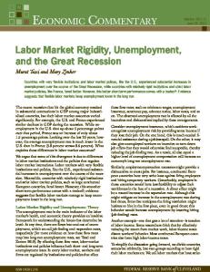
Measuring uncertainty is inherently difficult. Ideally, one would like to know the subjective probability distributions over future events from firms and households. As this is almost impossible to quantify directly, there exists no agreed measure of uncertainty in the literature and we have to rely on proxies. For our analysis, we take six widely-cited U.S. uncertainty measures from the literature. Considering this wide range of uncertainty proxies has the advantage that we are able to capture different kinds of uncertainty, such as (aggregate) macroeconomic uncertainty, financial uncertainty, economic policy uncertainty, and (idiosyncratic) firm-specific uncertainty. Specifically, the six uncertainty measures are (i) the macroeconomic uncertainty proxy proposed by Jurado et al. (2015), (ii) the financial uncertainty proxy proposed by Ludvigson et al. (2017), (iii) stock market volatility, (iv) corporate bond spreads, (v) a survey-based measure using the dispersion of firms’ forecasts about the general business outlook as a measure of (firm-specific) idiosyncratic uncertainty (Bachmann et al. 2013a,b), and (vi) the economic policy uncertainty index of Baker et al. (2016).5 Figure 1 presents the evolution of the six measures between January 1985 and December 2015. For comparison, each series has been demeaned and standardized; shaded areas mark recessions as dated by the NBER. Overall, the graphs are in line with well-known stylized facts concerning uncertainty proxies (see e.g. Bloom 2009). First, there is a sizeable degree of co-movement between the uncertainty indices. The positive unconditional correlation coefficients in Table 1 support this finding. Second, uncertainty is higher after political shocks like the 9/11 terrorist attack or Gulf War II. Third, the uncertainty proxies are predominantly countercyclical. Most of them increase noticeably before and during recessions while they are rather low during periods of stable economic expansion. 5

See Appendix A for more details on the construction of these measures.

4

Figure 1: U.S. uncertainty proxies 6 4

Black Monday

9/11

Gulf War I

Asian Crisis

Gulf War II

Debt Ceiling Dispute

2 0 −2 Macro Uncertainty Financial Uncertainty

−4

Russian & LTCM Default

−6 1985 6 4

1990

Black Monday

1995

2000

Worldcom & Enron

2005

9/11 Gulf War II

Gulf War I

Lehman

2010

Fiscal Cliff

2015

Debt Ceiling Dispute

Asian Crisis

2 0 −2 Russian & LTCM Default

Stock Market Volatility Corporate Bond Spread

−4

Worldcom & Enron

Lehman

Fiscal Cliff

−6 1985

1990

1995

2000

6 4

Black Monday

2005

9/11 Gulf War II

Gulf War I

2010

2015

Debt Ceiling Dispute

Asian Crisis

2 0 −2 −4

Forecast Disagreement Economic Policy Uncertainty

Russian & LTCM Default

Worldcom & Enron

Lehman

Fiscal Cliff

−6 1985

1990

1995

2000

2005

2010

2015

Notes: Each series has been demeaned and standardized by its standard deviation. The sample period is January 1985 to December 2015. Shaded areas mark recessions as dated by the NBER.

While these findings are interesting in itself, they provide no information about a causal effect of uncertainty on economic activity. We therefore have to resort to more sophisticated methods presented in the next subsection.

2.2

Empirical Model

Formally, we estimate the following VAR model on monthly data from January 19856 to December 2015: yt = µ + A(L)yt−1 + νt , 6

Determined by the availability of the EPU index.

5

(1)

Table 1: Cross-correlations

MU

FU

V XO

Spread

F DISP

EP U

Uncertainty proxies MU FU V XO Spread F DISP EP U

1

0.70*** 1

0.61*** 0.83*** 1

0.82*** 0.74*** 0.71*** 1

0.23*** 0.16** 0.23*** 0.22** 1

0.34*** 0.36*** 0.40*** 0.42*** 0.01 1

-0.16*** -0.08** 0.12 -0.25***

-0.10*** 0.68***

Activity variables ∆ log GDP UR

-0.18*** 0.11

-0.09** 0.06

-0.09* -0.01

Notes: Numbers are pairwise unconditional time-series correlation coefficients. Significance of correlation coefficients is tested via a nonparametric block bootstrap where *** denotes 1%, ** 5%, and * 10% significance levels, respectively. All variables are seasonally adjusted. Abbreviations: macro uncertainty (M U ), financial uncertainty (F U ), stock market volatility (V XO), corporate bond spread (Spread), forecast disagreement (F DISP ), and economic policy uncertainty (EP U ). The activity variables are the monthly growth rate of GDP (∆ log GDP ) and the unemployment rate (U R). The sample period is January 1985 to December 2015.

iid

where µ is a constant, A(L) is a lag polynomial of degree p = 12,7 and νt ∼ (0, Σ). The vector of endogenous variables yt comprises 12 variables and is similar in content to that used by Christiano et al. (2005) and Jurado et al. (2015). We choose such a large VAR to have a sufficiently large information set to correctly identify the structural shocks of interest and to capture a wide range of macroeconomic dynamics. In addition to the respective uncertainty proxy, the remaining 11 variables can be structured into four economic blocks, each one representing one relevant aspect of the economy. The first block represents the real economy, covering interpolated log GDP (see explanation below), log real consumption, and log real new orders (comprising new orders for consumer and capital goods). The second block contains quantity variables of the labor market namely log hours worked, the unemployment rate, and log employment. The third block captures price dynamics by adding the log of the personal consumption expenditures deflator and log real wages to our set of variables. And 7

Changing the number of lags to 6 or 24 has negligible qualitative or quantitative effects.

6

the fourth block represents money and financial market variables, covering the federal funds rate, the growth rate of M2, and the log S&P 500 index.8 One key issue for our analysis is the identification of exogenous movements in uncertainty. We follow Baker et al. (2016), Bloom (2009), Jurado et al. (2015), and a number of other papers in the uncertainty literature and employ a Cholesky-ordering. Specifically, we assume a lower-triangular matrix B, which maps reduced-form innovations νt into structural shocks εt .9 Bloom (2009) and Baker et al. (2016) impose the restriction that uncertainty does not react contemporaneously to movements in real activity, i.e. they order uncertainty first (or second after the S&P 500). Other authors, Jurado et al. (2015) most prominently, assume that the uncertainty proxy is contemporaneously affected by all other variables and hence ordered last in the recursive ordering in the VAR. This is more conservative in the sense that the uncertainty shock is the residual shock after all other shocks can act contemporaneously on the uncertainty proxy. As there is not much guidance from theory for the correct choice of ordering, we will use the Jurado et al. (2015)-ordering with uncertainty ordered last as our baseline and check the effect of different orderings in Section 5.1.10 Timing restrictions as the ones presented above are arguably too strong at the quarterly level, which is why we (and most of the uncertainty literature) employ a monthly VAR. However, GDP is not readily available at monthly frequency. Most monthly VAR studies therefore employ industrial production as a proxy for GDP. Manufacturing production, however, only accounts for about 12 percent of U.S. GDP and it seems reasonable to assume that other sectors might differ in their response to heightened uncertainty, e.g. in terms of 8

We will use the conceptual distinction of these blocks in a robustness check, where we separately exclude each block from the VAR (see Section 5.2). 9 Other approaches include Ludvigson et al. (2017), who propose a novel identification procedure by exploiting information from external variables and the timing of extraordinary economic events, and Benati (2014) who uses short- and medium-run restrictions in combination with sign restrictions. 10 While we are only interested in identifying uncertainty shocks and the ordering of the other variables is not crucial, one can give our ordering some economic intuition. By ordering the real economy first, we assume that it does not react contemporaneously to shocks in any other block. The labor block reacts contemporaneously to shocks in the real economy but not to price or financial shocks. Financial markets react immediately to shocks originating from the real economy or the labor market, however, they have no immediate impact on the real economy and the labor market.

7

adjustment costs for labor and capital or the dependence on external financing. Given that we are ultimately interested in the link between uncertainty and GDP, we decided to include an interpolated GDP series instead of industrial production. Until June 2010, we use the monthly GDP series provided by Stock and Watson (2010) and extend it to December 2015 by linking it to the monthly GDP estimate of Macroeconomic Advisers.11

3

Impulse response analysis

In this section we first look at the VAR dynamics following an uncertainty shock. The first row of Figure 2 depicts the estimated impulse response functions (IRFs) of GDP and the unemployment rate to a one-standard-deviation uncertainty shock.12 For all but one of the measures increases in uncertainty are accompanied by negative movements in GDP. The outlier is stock market volatility, where we do not find a negative reaction of GDP.13 While the GDP response to an economic policy uncertainty shock is not very pronounced, the responses to the four remaining uncertainty shocks are clearly negative and show similarities. In all cases the trough of -0.1 to -0.15 percent of GDP is reached after about a year. The persistence of the response, however, differs across the four measures, with macroeconomic and financial uncertainty showing the most persistent GDP effects. Overall, the GDP responses are very consistent with, e.g., Bachmann et al. (2013b) and Jurado et al. (2015),14 which is reassuring for our further analysis as the correct identification of the structural uncertainty shocks is crucial for quantifying the historical effects of exogenous uncertainty fluctuations. Heightened uncertainty has also been found to be partly responsible for the slow recovery 11

All sources are given in Table 6 in the appendix. Both monthly GDP series are very similar: the correlation between monthly growth rates for the overlapping period is above 0.9. 12 Other studies like Bloom (2009) and Jurado et al. (2015) report responses to four-standard-deviation shocks and obtain therefore more pronounced output declines. 13 This is in line with Choi (2013), who shows that sudden increases in stock market volatility have no impact on U.S. industrial production since the beginning of the Great Moderation. This might reflect that movements in stock market volatility are not only driven by uncertainty but also, to a large degree, by time-varying risk aversion (see, e.g., Bekaert et al. 2013). 14 Also consistent with these studies, we do not find the “wait-and-see” dynamics–an inital dip with a following overshoot–reported by Bloom (2009).

8

Figure 2: Uncertainty shocks in monthly VAR

Percent

GDP

GDP

0.2

0.2

0.1

0.1

0

0

−0.1

−0.1

−0.2

−0.2

−0.3

−0.3 Macro Uncertainty Corporate Bond Spread Stock Market Volatility

−0.4 −0.5

0

10

20

30

Financial Uncertainty Forecast Disagreement Economic Policy Uncertainty

−0.4

40

−0.5

50

0

10

Percentage points

Unemployment rate 0.25

0.2

0.2

0.15

0.15

0.1

0.1

0.05

0.05

0

0

−0.05

−0.05

−0.1

−0.1

−0.15

−0.15

−0.25

Macro Uncertainty Corporate Bond Spread Stock Market Volatility 0

10

20

30 Months

40

50

Financial Uncertainty Forecast Disagreement Economic Policy Uncertainty

−0.2 40

30

Unemployment rate

0.25

−0.2

20

−0.25

50

0

10

20

30 Months

40

50

Notes: IRFs of U.S. GDP and unemployment rate to one-standard-deviation uncertainty shocks derived from the monthly VAR including one of the six uncertainty measures (see text for details). Dark and light blue shaded areas: 68% and 95% confidence bands, respectively, constructed using a recursive design wild bootstrap (Goncalves and Kilian 2004) and reported for macro uncertainty and financial uncertainty.

of the U.S. labor market after the financial crisis (see, e.g., Leduc and Liu 2016). We indeed find for most uncertainty proxies that an exogenous increase in uncertainty is followed by a rise in unemployment (see the lower row of Figure 2). The macroeconomic uncertainty proxy and financial uncertainty proxy again show the largest effects, both in terms of magnitude and persistence. The maximum increase in the unemployment rate after an exogenous increase in macroeconomic uncertainty, for instance, is about 0.1 percentage points. Overall, the impulse response functions of the unemployment rate, depicted in the second row of Figure 2 are

9

consistent with our findings for GDP. The greater importance of the macroeconomic and financial uncertainty measures compared to the other proxies can also be seen in the variance decomposition reported in Table 7 in the appendix. Both macroeconomic and financial uncertainty explain up to 30 percent of the fluctuations in the unemployment rate horizons of one to two years. The other measures barely reach 10 percent. Our identified VAR also allows us to compute historical decompositions of the uncertainty proxies. Figure 3 plots the variation in the macroeconomic and financial uncertainty proxies, respectively, that is due to exogenous variation in uncertainty and contrasts it with the actual evolution of the proxies.15 The actual uncertainty proxies are only driven in small part by structural uncertainty shocks and seem to contain a large endogenous component due to other (first-moment) shocks.16 Figure 3: Historical decomposition of uncertainty measures

Macro Uncertainty

Financial Uncertainty

0.5 0.4

0.6 Exogenous Fluctuation Data

0.4

Exogenous Fluctuation Data

0.3 0.2

0.2

0.1

0

0 −0.2

−0.1 −0.2

−0.4

1990 1995 2000 2005 2010 2015

1990 1995 2000 2005 2010 2015

Notes: dashed blue line: part of fluctuation in macroeconomic uncertainty and financial uncertainty, resp., explained by corresponding structural uncertainty shocks. Solid black line: actual demeaned uncertainty measure.

15

The results for the other measures are similar but not reported for the sake of brevity. They are available upon request. The results further do not depend on the ordering of the uncertainty variable in the Cholesky decomposition of our VARs. 16 Cesa-Bianchi et al. (2014) also find that uncertainty is rather a symptom than a cause of macroeconomic instability.

10

4

Has higher uncertainty contributed to the Great Recession?

We are now in the position to quantify the impact of exogenous uncertainty fluctuations on U.S. GDP and unemployment since 2007. To this end, we compute a historical decomposition, which delivers, for each time period t and variable of interest i ∈ {gdp, unemp}, the estimated total effect of the sequence of identified historical uncertainty shocks. Formally, this decomposition is defined as

unc HIRFi,t =

t X

unc unc unc unc εbunc · IRFi,t−j = εbunc · IRFi,t + εbunc · IRFi,t−1 + . . . + εbunc · IRFi,0 , (2) j 0 1 t

j=0

unc where IRFi,h is the h-period-ahead impulse response of a shock today and εbunc is the t

estimated uncertainty shock in period t, e.g. January 2008. Both ingredients are based on the results in Section 3.17 GDP enters our empirical model in (monthly) log-levels, however, in our opinion, it is more instructive to study the contribution of exogenous uncertainty fluctuations to the quarter-onquarter growth rate of GDP. To do so, we first transform the monthly (log-)differences in unc HIRFgdp,t into an index

unc unc unc Igdp,t = Igdp,t−1 · (1 + ∆HIRFgdp,t ),

(3)

where the index is initialized at 1, and then calculate the growth rate of the quarterly averages of this index. For the unemployment rate, we are interested in the effect on the levels so the unc only transformation we conduct is to take quarterly averages of HIRFunemp,t to be consistent

with the depiction of quarter-on-quarter GDP growth. The first row of Figure 4 depicts the historical quarterly averages of macro uncertainty shocks (left column) and financial uncertainty shocks (right column) since 2007. The second 17 unc Note that this decomposition implies that HIRFi,t contains the impact of all uncertainty shocks since the beginning of our sample. Large shocks in the distant past could have an impact on our results today. We therefore run a robustness check where we restrict the IRF to zero after 96 months, i.e. roughly one business cycle. This has almost no effect on our baseline results. Results are available upon request.

11

Figure 4: Cumulative effects of structural uncertainty shocks on economic activity Macro Uncertainty Shocks

Financial Uncertainty Shocks

4

4

3

3

2

2

1

1

0

0

−1

−1

−2

−2

−3 2007Q1

2009Q1

2011Q1

2013Q1

−3 2007Q1

2015Q1

2009Q1

Percentage Points

GDP Growth 2

1

1

0

0

−1

−1

−2

2009Q1

2011Q1

2013Q1

−3 −4 2007Q1

2015Q1

2009Q1

Unemployment Rate

Percentage Points

2015Q1

−2 GDP growth (qoq) Uncertainty Contribution

−3

2011Q1

2013Q1

2015Q1

Unemployment Rate

6

6

4

4

2

2

0

0 Unemployment Rate Uncertainty Contribution

−2 2007Q1

2013Q1

GDP Growth

2

−4 2007Q1

2011Q1

2009Q1

2011Q1

2013Q1

−2

2015Q1

2007Q1

2009Q1

2011Q1

2013Q1

2015Q1

Notes: Left column: contributions of macro uncertainty shocks; right column: contributions of economic policy uncertainty shocks. The blue thin bars display the cumulative effects of the structural uncertainty shocks. The beige thick bars show the actual realizations. Actual realizations of GDP growth are defined as the demeaned quarter-on-quarter GDP growth rates (second row). Actual realizations of unemployment rate are defined as differences to the unemployment rate in 2007Q1 (third row). Shock series in the first row are normalized by their standard deviation.

(third) row shows the results for GDP growth (the unemployment rate), where the effects of the structural uncertainty shocks are depicted by the blue thin bars and the observed activity variable by beige thick bars. To obtain the latter we demean the quarter-on-quarter GDP growth rates. For the unemployment rate we use the difference between the actual outcome in period t and the fixed value of the first quarter of 2007.Visual inspection of the graphs suggests that the exogenous increases in both macroeconomic and financial uncertainty have contributed to the Great Recession only to a limited extent. Both, however, seem to have 12

played a role in the persistently high unemployment rates in 2010 and 2011, although the quantitative effects are minor. Table 2 reports the annual contributions to GDP growth and the unemployment rate for all uncertainty measures in our sample. For most uncertainty measures, we find a dampening effect on economic activity during the Great Recession, albeit a small one. Financial uncertainty, for example, had a total negative impact on GDP growth of 0.3 percentage points in 2009 and macroeconomic uncertainty exhibits negative effects of 0.2 percentage points both in 2008 and 2009. So, even at the height of the crisis, uncertainty cannot explain a major part of the drop in GDP. The results are broadly consistent for the other uncertainty measures. They deliver negative growth contributions in the range of 0.1 to 0.5 percentage points over the years 2008 and 2009.18 Regarding the unemployment rate, we are particularly interested in examining the role of uncertainty for the “jobless recovery”, which is characterized by a persistently high level of unemployment after the crisis. The lower panel of Table 2 reports the contribution of exogenous uncertainty fluctuations to the rise in the level of unemployment rate since 2007. Our results support the view that second moment shocks might be a factor for the “jobless recovery” after the crisis. They, however, do not seem to be the major driver. The largest effects stem from financial uncertainty shocks that are able to explain 0.7 percentage points of the overall increase of 4.3 percentage in the unemployment rate in 2011 compared to 2007. Overall, our results support the view that higher uncertainty was more a concomitant of bad negative first moment shocks rather than a cause of the Great Recession and the subsequent “jobless recovery”. 18

The small role that economic policy uncertainty played in the Great Recession is in line with the findings of Benati (2014), who conducts a thorough analysis of the effects of policy uncertainty in the Great Recession and finds small effects not only for the U.S. but also for the UK, Canada, and the Euro area. However, to the extent that the EPU index is more focused on fiscal uncertainty, it might understate the effects of monetary policy uncertainty since 2007. We therefore also use (i) a sub-index of the Baker et al. (2016)-EPU index focusing on word counts related to monetary policy uncertainty and (ii) a new index constructed by the Fed (Husted et al. 2016) also based on word counts but with a cleaner focus on monetary policy uncertainty. Using either index leads to a non-negative response of GDP and a fall in the unemployment rate. Results are available upon request.

13

Table 2: Contributions of uncertainty shocks to U.S. economic activity from 2008 to 2015

Years

MU

FU

V XO

Spread

F DISP

EP U

Actual Realizations

0.1 0.2 0.2 0.0 -0.2 -0.5 -0.2 -0.1

-0.1 -0.5 0.1 0.0 0.2 0.2 0.3 0.1

0.0 -0.3 0.0 0.0 0.3 0.1 0.2 -0.1

-0.2 -0.1 0.2 0.1 0.1 -0.1 0.1 0.4

-2.9 -5.3 0.0 -1.0 -0.3 -0.9 -0.2 0.0

0.2 0.4 0.3 0.4 0.5 0.6 0.6 0.5

0.1 0.3 0.3 0.3 0.1 0.0 -0.2 -0.3

0.0 0.1 0.2 0.1 0.0 -0.1 -0.3 -0.2

0.1 0.1 0.0 -0.1 -0.1 -0.1 -0.2 -0.2

1.2 4.7 5.0 4.3 3.5 2.8 1.6 0.7

GDP growth 2008 -0.2 0.0 2009 -0.2 -0.3 2010 0.1 0.0 2011 0.1 -0.2 2012 0.2 0.1 2013 -0.1 0.0 2014 0.3 0.3 2015 -0.4 -0.2 U nemplyoment rate 2008 0.1 0.0 2009 0.3 0.3 2010 0.4 0.5 2011 0.4 0.7 2012 0.1 0.5 2013 0.2 0.4 2014 -0.1 -0.1 2015 0.0 -0.1

Notes: Growth contributions (in percentage points) of the respective structural uncertainty shocks to annual GDP growth and the unemployment rate. Abbreviations: macro uncertainty (M U ), financial uncertainty (F U ), stock market volatility (V XO), corporate bond spread (Spread), forecast disagreement (F DISP ), and economic policy uncertainty (EP U ). Actual realizations of GDP growth are defined as the actual demeaned GDP growth rates. Actual realizations of unemployment rate are defined as differences to the unemployment rate in 2007.

5

Robustness and extensions

To corroborate our baseline results we now perform a number of robustness checks. We (i) change the ordering of the uncertainty measure in the Cholesky identification scheme of the structural shocks, (ii) we leave out certain blocks of variables, (iiii) we estimate the effects of each uncertainty measure on the longest available sample, and (iv) we use a two-step approach as another option to study the effects of the monthly structural uncertainty shocks on quarterly GDP growth. 14

5.1

Ordering of the uncertainty proxy

In our first robustness check, we analyze the importance of our decision to order the uncertainty proxy last in our baseline VAR. Ordering it last means that the uncertainty proxy is affected by all other shocks originating from the SVAR contemporaneously, whereas uncertainty shocks can affect the other variables only with a one period lag. To check the robustness of this identification assumption, we redo our analysis for the other 11 possible positions of the uncertainty measure within the recursive identification scheme, where we leave the other variables in their relative ordering unchanged. For the sake of brevity we only show the results for macro and financial uncertainty in Figure 5.19 The shaded area gives the range of uncertainty contributions for the different orderings. It can clearly be seen that our results are not substantially affected by the position of the uncertainty proxy within the recursive identification scheme. For both GDP growth and the unemployment rate, the estimated effects are within a very small band around our baseline results.

5.2

Excluding certain blocks of variables

A natural question in VAR studies is always which variables to include. The goal of our large 12-variable baseline VAR is to make the information set rich enough to properly identify uncertainty shocks and to not omit important dynamics. In this robustness check, we analyze how omitting certain groups of variables affects our results. We conduct four different experiments. In each of them we exclude one of the blocks described in Section 2.2 from our VAR and redo the computation of historical uncertainty contributions.20 We again only show the results for macro and financial uncertainty as representative examples in Figure 6. On average, the resulting uncertainty contributions increase when we omit variables from the VAR. Intuitively, these larger estimates are not surprising as our shocks might now pick up fluctuations that where controlled for by the additional observables 19

The outcomes are very similar for the other uncertainty measures. Note that our two main variables of interest, GDP and the unemployment rate, are never excluded. E.g. in the first experiment, we exclude the real variables (real consumption and real orders) but not real GDP. 20

15

Figure 5: Robustness check: alternative orderings of the uncertainty proxy

GDP Growth (Percentage Points)

Macro Uncertainty 2

1

1

0

0

−1

−1

−2

−2

−3

−3

−4 −5 −6

Unemployment Rate (Percentage Points)

Financial Uncertainty

2

−4 Actual Baseline Interval Different Orderings

−5 −6

2008 2009 2010 2011 2012 2013 2014 2015

6

6

5

5

4

4

3

3

2

2

1

1

0

0

−1

−1

−2

−2

2008 2009 2010 2011 2012 2013 2014 2015

2008 2009 2010 2011 2012 2013 2014 2015

2008 2009 2010 2011 2012 2013 2014 2015

Notes: Annual cumulative effects of structural uncertainty shocks on economic activity. Left column: contributions of macro uncertainty shocks; right column: contributions of financial uncertainty shocks. Black solid lines display the baseline cumulative effects of the structural uncertainty shocks. The white bars show the actual realizations. Actual realizations of GDP growth are defined as the demeaned annual GDP growth rates (first row). Actual realizations of unemployment rate are defined as differences to the unemployment rate in 2007 (second row). Shaded areas contain the cumulative effects determined with all possible different orderings of the uncertainty proxies in the recursive identification approach (holding the relative positions of the other variables constant).

in the baseline model. For example, when excluding the price variables, the maximum contribution of macroeconomic uncertainty rises to about minus 1 percentage point in 2009. This is considerably above the baseline results. Overall, given the actual GDP decline of minus 5 percent in 2009 for instance, even the maximum contributions in this robustness check are still limited. Our main findings therefore do not change. Even though the importance of uncertainty increases somewhat, we 16

cannot find evidence for exogenous uncertainty fluctuations being a main driver of the Great Recession. Figure 6: Robustness check: exclusion of certain blocks of variables

GDP Growth (Percentage Points)

Macro Uncertainty 2

1

1

0

0

−1

−1

−2

−2

−3 −4

−6

−3

Data Baseline w/o Real Variables w/o Labor Market Variables w/o Price Variables w/o Financial Variables

−5

Unemployment Rate (Percentage Points)

Financial Uncertainty

2

−4 −5 −6

2008 2009 2010 2011 2012 2013 2014 2015

6

6

5

5

4

4

3

3

2

2

1

1

0

0

−1

−1

−2

−2

2008 2009 2010 2011 2012 2013 2014 2015

2008 2009 2010 2011 2012 2013 2014 2015

2008 2009 2010 2011 2012 2013 2014 2015

Notes: Annual cumulative effects of structural uncertainty shocks on economic activity. Left column: contributions of macro uncertainty shocks; right column: contributions of financial uncertainty shocks. Black solid lines display the cumulative effects of the structural uncertainty shocks of our baseline estimates. The white bars show the actual realizations. Actual realizations of GDP growth are defined as the demeaned annual GDP growth rates (first row). Actual realizations of unemployment rate are defined as differences to the unemployment rate in 2007 (second row). The other lines depict the results for the SVARs without certain blocks of variables.

5.3

Prolonged sample

In our third robustness check, we extend the length of our estimation sample. In our baseline scenario, we started all estimations in January 1985 as the economic policy uncertainty is 17

not available earlier. One may, however, argue that the more volatile times of the 1970s and early 1980s carry important information for our analysis. We therefore now use the longest available samples for each uncertainty proxy. The specific starting dates can be found in Table 5 in the appendix. Table 3 provides the contributions of the uncertainty shocks to GDP growth and the unemployment rate for the years from 2008 to 2015. It is apparent that especially for macroeconomic and financial uncertainty the detrimental effects on GDP get considerably larger (not so much for the other measures). Macroeconomic uncertainty explains 2.2 percentage points of the drop in U.S. GDP growth in 2009. This finding also holds true for the unemployment rate. About half of the increase in unemployment can be explained by the effects of uncertainty determined with this proxy. In our view there are two reasons why in this exercise uncertainty shocks cause larger fluctuations in U.S. GDP and in the unemployment rate. First, compared to the baseline calculations the estimations of this robustness check provide in general larger negative impulse unc response functions, IRFi,t , to a given uncertainty shock in macroeconomic and financial

uncertainty. This observation squares well with the results of Choi (forthcoming) and Mumtaz and Theodoridis (forthcoming) who show that the impact of uncertainty shocks on the U.S. real economy has declined over time. They explain this with a more aggressive response of U.S. monetary policy to changes in inflation and a flattening of the Phillips curve. According to these explanations the negative growth contributions in Table 3 are presumably overstated. Second, the calculations based on the prolonged sample deliver much larger positive historical uncertainty shocks, εbunc t , in the years 2007 and 2008 compared to the baseline scenario. One explanation could lie in structural breaks within the structural uncertainty equation of the SVAR. To investigate this, we separately estimate the structural uncertainty equation of our VAR, i.e. the equation relating the uncertainty proxy to its own lags and the contemporaneous values as well as the lags of the other endogenous variables. In the long sample, we find that classical statistical tests (e.g. CUSUM squared) reject the stability of

18

the estimated coefficients in the case of macroeconomic and financial uncertainty. In contrast to this using as estimation starting point January 1985 delivers stable coefficients.21 This gives us confidence that the quantitative effects of exogenous uncertainty fluctuations lie presumably more in the range of our baseline estimates. Table 3: Robustness check: long sample contributions of uncertainty shocks to U.S. economic activity from 2008 to 2015

V XO

Spread

F DISP

EP U

Actual Realizations

GDP growth 2008 -0.9 -0.5 2009 -2.2 -2.4 2010 -0.8 -0.6 2011 -0.4 0.0 2012 1.3 0.6 2013 1.3 1.5 2014 1.1 0.7 2015 -0.5 0.1

0.2 0.1 0.1 -0.2 0.1 -0.1 0.2 0.2

-0.3 0.6 0.5 -0.1 -0.2 0.0 -0.2 -0.3

-0.2 -0.4 -0.5 -0.3 0.0 0.3 0.5 0.5

-0.2 -0.1 0.2 0.1 0.1 -0.1 0.1 0.4

-2.9 -5.3 0.0 -1.0 -0.3 -0.9 -0.2 0.0

U nemplyoment rate 2008 0.4 0.4 2009 2.0 2.0 2010 2.5 2.6 2011 2.5 2.4 2012 1.7 1.8 2013 0.8 0.7 2014 0.1 0.1 2015 0.2 0.0

0.0 0.1 0.2 0.3 0.3 0.2 0.0 -0.2

0.1 -0.1 -0.4 -0.3 -0.2 -0.1 0.0 0.1

0.1 0.4 0.7 0.8 0.7 0.5 0.1 -0.2

0.1 0.1 0.0 -0.1 -0.1 -0.1 -0.2 -0.2

1.2 4.7 5.0 4.3 3.5 2.8 1.6 0.7

Years

MU

FU

Notes: Growth contributions (in percentage points) of the respective structural uncertainty shocks to annual GDP growth and the unemployment rate. Abbreviations: macro uncertainty (M U ), financial uncertainty (F U ), stock market volatility (V XO), corporate bond spread (Spread), forecast disagreement (F DISP ), and economic policy uncertainty (EP U ). Actual realizations of GDP growth are defined as the actual demeaned GDP growth rates. Actual realizations of unemployment rate are defined as differences to the unemployment rate in 2007. Estimation sample is the longest available sample for each uncertainty proxy (see Table 5).

21

All results available from the authors on request.

19

5.4

Two-stage estimation approach

So far we performed our complete analysis in one single step by estimating monthly VARs, where we used a monthly interpolated GDP time series. Kilian (2009), however, raises the issue that such an interpolated time series can cause spurious dynamics. To circumvent this issue, he proposes a two-step estimation approach which we employ in our final robustness check.22 In the first step we identify structural uncertainty shocks via monthly VARs. We modify our baseline VARs in two points: (i) we include industrial production and (ii) drop monthly GDP and the unemployment rate. The uncertainty proxy is again ordered last and we identify the VAR recursively, i.e. the model corresponds one-to-one to the VAR in Jurado et al. (2015). We estimate the VAR using monthly data from January 1985 onwards. Our benchmark estimation includes 12 lags. In the second step, we take the identified structural uncertainty shocks and employ them to explain fluctuations of quarter-on-quarter GDP growth rates and quarterly unemployment rates. To this end, we first calculate quarterly averages of the monthly uncertainty innovations, say, e¯t , and then estimate a regression of the form

qt = α +

12 X

φi e¯t−i + εt .

(4)

i=0

By including the contemporaneous value of e¯t we assume that our first stage uncertainty innovations are predetermined within the same quarter with respect to GDP or the unemployment rate which seems plausible after our identification procedure in the first stage. To obtain an estimate of the quantitative impact of exogenous fluctuations on the U.S. economy since 2007, we therefore proceed as follows: first, we calculate for each uncertainty measure the quarterly averages of the identified monthly structural uncertainty shocks from the VARs. In a second step, we use the quarterly regression model (4) and the historical quarterly uncertainty shocks to compute the predicted historical values for GDP 22

Meinen and Röhe (2017) also use that approach to analyze the effects of uncertainty on investment in France, Germany, Italy and Spain.

20

growth and the unemployment rate. As an example, we compute the predicted value for GDP growth for the first quarter in 2010, qb2010q1 , given the quarterly averages of structural shocks, e¯, as: b e b ¯ b ¯ b+φ qb2010q1 = α 0 ¯2010q1 + φ1 e 2009q4 + . . . + φ12 e 2007q1 .

(5)

The predicted values enable us to study the cumulative effects of the structural uncertainty shocks on GDP growth and the unemployment rate, i.e. we obtain a historical decomposition. Table 4 reports the contributions to GDP growth and the unemployment rate for each uncertainty measure. Overall, the uncertainty contributions are not too different to the baseline, albeit slightly larger. We conclude that the interpolation of GDP to a monthly series is not driving our results.

21

Table 4: Robustness check: two-stage estimation approach contributions of uncertainty shocks to U.S. economic activity from 2008 to 2015

V XO

Spread

F DISP

EP U

Actual Realizations

GDP growth 2008 0.0 0.0 2009 -0.6 -0.5 2010 -0.1 -0.1 2011 0.3 -0.5 2012 0.6 0.2 2013 0.3 0.0 2014 0.2 0.2 2015 -0.3 0.3

0.1 -0.2 0.0 0.1 -0.1 0.1 0.1 0.0

0.0 -0.3 -0.7 -0.4 -0.2 -0.1 0.4 0.4

0.2 -0.8 -0.4 -0.5 0.4 -0.2 0.0 0.6

-0.7 -0.9 0.6 -0.1 0.4 -0.3 0.7 1.6

-2.9 -5.3 0.0 -1.0 -0.3 -0.9 -0.2 0.0

U nemplyoment rate 2008 0.0 0.0 2009 0.5 0.6 2010 1.0 1.1 2011 0.6 1.0 2012 0.2 0.6 2013 0.0 0.0 2014 -0.4 -0.5 2015 -0.6 -0.7

0.0 0.5 0.7 0.6 0.3 0.1 -0.5 -0.5

0.0 0.5 1.0 0.6 0.2 0.0 -0.4 -0.6

-0.2 0.6 1.3 1.2 0.0 0.2 -0.1 -0.6

0.0 0.6 1.1 1.0 0.6 0.0 -0.5 -0.7

1.2 4.7 5.0 4.3 3.5 2.8 1.6 0.7

Years

MU

FU

Notes: Growth contributions (in percentage points) of the respective structural uncertainty shocks to annual GDP growth and the unemployment rate. Abbreviations: macro uncertainty (M U ), financial uncertainty (F U ), stock market volatility (V XO), corporate bond spread (Spread), forecast disagreement (F DISP ), and economic policy uncertainty (EP U ). Actual realizations of GDP growth are defined as the actual demeaned GDP growth rates. Actual realizations of unemployment rate are defined as differences to the unemployment rate in 2007.

22

6

Conclusion

In this paper we estimated the quantitative impact of exogenous fluctuations in uncertainty on U.S. GDP and the unemployment rate in the Great Recession and the ensuing recovery. To do so, we studied the effects of shocks derived from six different uncertainty proxies in monthly VARs and computed historical decompositions. We found that, first, only a minor part of the rise in uncertainty measures during the crisis was driven by exogenous uncertainty shocks. Second, our results showed that uncertainty shocks can explain about 10 percent of the drop in GDP (from trend) at the height of the crisis. However, the different uncertainty shock measures vary considerably in their effects. Interestingly, our analysis suggests that financial uncertainty shocks increased the unemployment rate by 0.5 to 0.7 percentage points in 2010 and 2011. Financial uncertainty might therefore be a candidate to explain parts of the slow recovery of the labor market after the crisis. Our results are broadly robust across different uncertainty proxies and model specifications. Excluding blocks of variables from the VAR or increasing the sample length to include the volatile times of the 1970s and early 1980s increased the estimated contributions somewhat. What we are potentially missing from our analysis are non-linearities related to the zero lower bound for the nominal interest rate. Using DSGE models including a zero lower bound for the nominal interest rate, Johannsen (2014) and Fernández-Villaverde et al. (2015) find that the effects of fiscal policy uncertainty are amplified when the central bank is constrained. This question is left for future research.

23

References Bachmann, Rüdiger, Benjamin Born, Steffen Elstner, and Christian Grimme (2013a). “Timevarying business volatility, price setting, and the real effects of monetary policy”. CEPR Discussion Paper 9702. Bachmann, Rüdiger, Steffen Elstner, and Eric R. Sims (2013b). “Uncertainty and economic activity: evidence from business survey data”. American Economic Journal: Macroeconomics 5 (2), 217–249. Baker, Scott R., Nicholas Bloom, and Steven J. Davis (2016). “Measuring economic policy uncertainty”. Quarterly Journal of Economics 131 (4), 1593–1636. Bekaert, Geert, Marie Hoerova, and Marco Lo Duca (2013). “Risk, uncertainty and monetary policy”. Journal of Monetary Economics 60 (7), 771 –788. Benati, Luca (2014). “Economic policy uncertainty and the great recession”. University of Bern, mimeo. Bloom, Nicholas (2009). “The impact of uncertainty shocks”. Econometrica 77 (3), 623–685. (2014). “Fluctuations in uncertainty”. Journal of Economic Perspectives 28 (2), 153–76. Born, Benjamin and Johannes Pfeifer (2014). “Policy risk and the business cycle”. Journal of Monetary Economics 68, 68–85. Cesa-Bianchi, Ambrogio, M. Hashem Pesaran, and Alessandro Rebucci (2014). “Uncertainty and economic activity: a global perspective”. CESifo Working Paper Series 4736. Choi, Sangyup (2013). “Are the effects of Bloom’s uncertainty shocks robust?” Economics Letters 119 (2), 216–220. (forthcoming). “Variability in the effects of uncertainty shocks: new stylized facts from OECD countries”. Journal of Macroeconomics. Christiano, Lawrence J., Martin Eichenbaum, and Charles L. Evans (2005). “Nominal rigidities and the dynamic effects of a shock to monetary policy”. Journal of Political Economy 113 (1), 1–45. Fernández-Villaverde, Jesús, Pablo A. Guerrón-Quintana, Keith Kuester, and Juan F. RubioRamírez (2015). “Fiscal volatility shocks and economic activity”. Amercian Economic Review 105 (11), 3352–3384. Goncalves, Silvia and Lutz Kilian (2004). “Bootstrapping autoregressions with conditional heteroskedasticity of unknown form”. Journal of Econometrics 123 (1), 89–120. Husted, Lucas, John Rogers, and Bo Sun (2016). “Measuring monetary policy uncertainty: the Federal Reserve, January 1985-January 2016”. IFDP Notes 2016-04-11. Federal Reserve Board.

24

Johannsen, Benjamin K. (2014). “When are the effects of fiscal policy uncertainty large?” Finance and Economics Discussion Series 2014-40. Federal Reserve Board. Jurado, Kyle, Sydney C. Ludvigson, and Serena Ng (2015). “Measuring uncertainty”. American Economic Review 105 (3), 1177–1216. Kilian, Lutz (2009). “Not all oil price shocks are alike: disentangling demand and supply shocks in the crude oil market”. American Economic Review 99 (3), 1053–69. Leduc, Sylvain and Zheng Liu (2016). “Uncertainty shocks are aggregate demand shocks”. Journal of Monetary Economics 82, 20–35. Ludvigson, Sydney C., Sai Ma, and Serena Ng (2017). “Uncertainty and business cycles: exogenous impulse or endogenous response?” Working Paper, New York University. Meinen, Philipp and Oke Röhe (2017). “On measuring uncertainty and its impact on investment: cross-country evidence from the euro area”. European Economic Review 92, 161–179. Mumtaz, Haroon and Paolo Surico (2015). “The transmission mechanism in good and bad times”. International Economic Review 56 (4), 1237–1260. Mumtaz, Haroon and Konstantinos Theodoridis (forthcoming). “The changing transmission of uncertainty shocks in the U.S.” Journal of Business & Economic Statistics, 1–14. Mumtaz, Haroon and Francesco Zanetti (2013). “The impact of the volatility of monetary policy shocks”. Journal of Money, Credit and Banking 45 (4), 535–558. Stock, James H. and Mark W. Watson (2010). “Distribution of quarterly values of GDP/GDI across months within the quarter”. Research Memorandom.

25

A

Data Sources Table 5: U.S. uncertainty measures: description and sources

Variable

Description

Source

Macro Uncertainty (M U )

common factor of three-months ahead forecast error variance de- Jurado composition; available since 7/1960 (2015)

Financial Uncertainty (F U )

common factor of three-months ahead forecast error variance de- Ludvigson et al. composition; available since 7/1960 (2017)

Stock Market Volatility (V XO)

concatenated series of the monthly volatility of daily S&P 500 returns (from 1/1957 to 12/1985) and the implied volatility index from options (VXO) (since 1/1986)

S&P

Corporate Bond Spread (SP READ)

spread of the 30-year Baa-rated corporate bond yield index over the 30-year treasury bond yield; in months where the 30-year treasury bond was missing the 20-year treasury bond was used; available since 4/1953

Federal Reserve Board

Forecast Disagreement (F DISP )

cross-sectional standard deviation of BOS general business expectation question; manufacturing, third FED district, seasonally adjusted; available since 5/1968

BOS

Economic Policy Uncertainty (EP U )

aggregation of four components: a scaled count of news articles Baker that refer to the economy, uncertainty and policy; discounted dollar- (2016) weighted sum of scheduled expirations of federal tax code provisions; and indexes of disagreement among professional forecasters about future CPI inflation and about future government purchases of goods and services; available since 1/1985

et

et

al.

al.

Notes: All series were downloaded from the cited sources in March 2017 at the most recent vintage available at that time. While SP READ is available since 4/1953, our earliest regressions start in January 1959 as the interpolated monthly GDP series is not available earlier.

26

Table 6: Additional U.S. variables: description and source Variable

Description

Source

Gross Domestic Product (monthly)

billions of chained 2009 dollars, monthly, seasonally adjusted, Stock/Watson monthly real GDP (from 1/1959 - 6/2010) extended by growth rates of the Macro Advisors monthly real GDP (from 7/2010 - 12/2015); the time series of Stock and Watson is available at http://www.princeton.edu/~mwatson/mgdp_gdi.html.

Mark Watson and Macroeconomic Advisors

Gross Domestic Product (quarterly)

billions of chained 2009 dollars, quarterly, seasonally adjusted

Federal Reserve Bank St. Louis

Industrial duction

index (2012=100), monthly, total industry, seasonally adjusted

FRED MD

Real Consumption

index (2009=100), monthly, real personal consumption expenditures, seasonally adjusted

FRED MD

Real Orders

millions of chained 2009 dollars , monthly, orders for consumer goods and capital goods deflated by price index of personal consumption expenditure, seasonally adjusted

Conference Board

Hours

hours, monthly, average weekly hours in manufacturing, seasonally adjusted

FRED MD

Unemployment Rate

percent, monthly, civilian unemployment rate, seasonally adjusted

FRED MD

Employment

million persons, monthly, all employees total nonfarm, seasonally adjusted

FRED MD

Consumer Prices

index (2009=100), monthly, personal consumption expenditure, seasonally adjusted

FRED MD

Real Wages

chained 2009 dollars, monthly, average hourly earnings in manufacturing deflated by price index of personal consumption expenditure, seasonally adjusted

FRED MD

Federal Rate

percent, monthly, effective federal funds rate

FRED MD

Broad Money

billions of dollars, monthly, M2 money stock

FRED MD

Stock Index

common S&P 500 stock price index, composite

FRED MD

Pro-

Funds

Notes: All series were downloaded from the cited sources in March 2017 at the most recent vintage available at that time.

27

B

Variance Decomposition Table 7: Variance Decomposition

Horizon

MU

FU

V XO

Spread

F DISP

EP U

0.0% 8.0% 8.8% 7.3% 5.0% 4.0%

0.0% 7.2% 7.9% 7.6% 5.9% 5.4%

0.0% 1.3% 3.5% 3.6% 2.3% 1.9%

0.0% 11.7% 9.8% 7.9% 5.4% 4.2%

0.0% 12.0% 11.1% 7.6% 4.9% 3.6%

0.0% 1.4% 1.5% 1.1% 1.4% 1.7%

0.0% 31.2% 24.8% 19.4% 13.0% 9.6%

0.0% 25.3% 28.7% 26.3% 18.3% 13.7%

0.0% 3.0% 2.2% 1.6% 1.3% 2.7%

0.0% 10.7% 9.3% 6.6% 4.1% 3.2%

0.0% 8.1% 9.9% 6.8% 4.2% 3.0%

0.0% 0.8% 0.3% 1.0% 2.3% 3.0%

M anuf acturing P roduction GDP h=1 h = 12 h = 24 h = 36 h = 48 h = 60 U nemploymentRate h=1 h = 12 h = 24 h = 36 h = 48 h = 60

Notes: The VAR consists of log interpolated GDP, log real consumption, log real new orders, log hours worked, the unemployment rate, log employment, log PCE deflator, log real wages, the federal funds rate, the growth rate of M2, the log S&P 500 index, and one of the following six uncertainty measures: macro uncertainty (M U ), financial uncertainty (F U ), stock market volatility (V XO), corporate bond spread (Spread), forecast disagreement (F DISP ), and economic policy uncertainty (EP U ). The VARs are estimated separately with 12 lags and a constant. To compute the variance decomposition we assume that the uncertainty measure is ordered last. The sample period is January 1985 to December 2015.

28