Understanding the Great Recession

Lawrence Christiano

Martin Eichenbaum

Mathias Trabandt

August 25, 2014

Disclaimer: The views expressed are those of the authors and not necessarily those of the Federal Reserve Board or any other person associated with the Federal Reserve System.

The Great Recession and its Aftermath ! Extraordinary contractions in GDP, investment and

consumption.

! Employment and labor force participation dropped substantially,

with little/no recovery.

! Vacancies recovered but unemployment still above pre-recession

levels (ëshift in Beveridge curveí).

! Despite severe economic weakness, decline in ináation relatively

modest.

Questions

1

What were key forces driving U.S. economy during the Great Recession?

2

Mismatch in the labor market?

3

Why was the drop in ináation so moderate?

Answering our Questions requires a Model ! Model must provide empirically plausible account of: ñ standard macro- and labor market data. ! Novel features of labor market ñ Endogenize labor force participation. ñ Derive wage inertia as an equilibrium outcome. ! Estimate model using pre-2008 data. ! Use estimated model to analyze post-2008 data.

Questions and Answers ! What forces drove real quantities in the Great Recession? ñ Shocks to Önancial markets key drivers, even for variables like labor force participation. ñ Government shocks not important: because of size and timing (consistent with ZLB literature). ! Mismatch in the labor market? ñ Not a Örst order feature of the Great Recession. ñ We account for ëshiftí in the Beveridge curve without resorting to structural shifts in the labor market.

Questions and Answers

! Why was the drop in ináation so moderate? ñ Prolonged slowdown in TFP growth during the Great Recession. ñ Rise in cost of Örmsí working capital as measured by spread between corporate-borrowing rate and risk-free interest rate. ñ Both forces excert countervailing pressure on ináation.

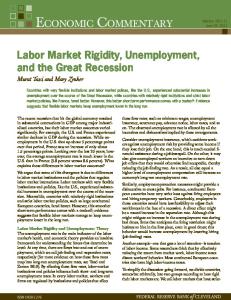
Labor Market

Employment* E*

Unemployment* U*

Non,par/cipa/on* N*

om the household. All workers have the same concave preferences optimal insurance arrangement involves allocating the same level he home good to all members of the household. usehold maximizes the objective function:

Labor Market

E0

1 X t=0

 t U(C~t );

Employment* E*

h " #" i !1 " C~t = (1 ! !) (Ct~)1 + ! CtH

~ = U(C)

CtH = 1 ! Lt

C

1 ; 1

      1 H (1  !) Ct  bCt1 + ! CtH  bCt1 :

(2.8)

(2.9)

market consumption and the consumption of a good produced at Non,par/cipa/on* Unemployment* governs the substitutability between Ct and CtH : In the next draft N* U* t results for other values of . The parameter b controls the degree sehold preferences. We assume 0  b < 1: A bar over a variable ,Household*labor*force*decision* ,Split*between*U*and*E*determined*by*job,finding*rate.* e average value.

f the household. Workers maximize expected income in exchange for perfect nsurance from the household. All workers have the same concave preferences h " #" i " C~t = (1 ! !) (Ct ) + ! CtH tion. So the optimal insurance arrangement involves allocating the same level 1!$ $ CtHand = (1 ! Lt )home (Lt good ! lt ) to all members of the household. good the entative household hmaximizes the objective function: Pt Ct + PI;t It + Bt+1 i1

Labor Market

1 !

c

c

" ~PttD= RK;t Kt + (Lt ! lt )C Wt ! + R!) B t + lt(1 t!11 t! (C t )Tt

X

t

" #" + ! CtH

!

~

E0  U(Ct ); max 1!$c H;It ;lt g1 fCt ;Lt ;CtH ;Bt+1 ;K t=0 Ct+1 Lt ) (Lt t = (1 ! t=0

$ !Employment* lt ) c E*

C~ 1  1 CtH P= LtIt +~ Bt+1 +!PI;t t Ct 1 U(C) = ;  Kt+1 (1t ! Ktlt+ " R=K;t K + $(L ) PIt1D K t) ! t + lt Wt + Rt!1 Bt ! Tt

(2.8)

(2.9)

      1 H KC~t+1 = (1 ! $ ) K +Imax t + ! CtH1 bCt1 : t = (1  !) KCt t bCt1 H fCt ;Lt ;Ct ;Bt+1 ;Kt+1 ;It ;lt gt=0 CtH denote market consumption and the consumption of a good produced at rameter, ; governs the substitutability between Ct and CtH : In the next draft e will report results for other values of . The parameter b controls the degree Non,par/cipa/on* Unemployment* ation in household preferences. We assume 0  b < 1: A bar over a variable N* U* conomy-wide average value. 5

,Household*labor*force*decision* ,Split*between*U*and*E*determined*by*job,finding*rate.*

Labor Market

Employment* E*

Unemployment* U*

Non,par/cipa/on* N*

Bargaining* Three*types*of*worker,firm*mee/ngs:* *i)*E*to*E*,*ii)*U*to*E,*iii)*N*to*E**

Alternating O§er Bargaining (AOB) ! Firms pay a Öxed cost to meet a worker. ! Then, workers and Örms bargain. ñ Disagreement leads to continued negotiations ! Hall-Milgrom (2008): if bargaining costs donít depend

sensitively on state of economy, neither will wages.

! CET (2013): AOB outperforms Nash bargaining in empirical

NK model (no Shimer puzzle)

ñ after expansionary shock, rise in wages relatively small leading to substantial ampliÖcation.

Estimated Medium-Sized DSGE Model ! Standard empirical NK model (e.g., CEE, ACEL, SW): ñ ñ ñ ñ ñ ñ

Calvo price setting frictions, but no indexation. Habit persistence. Variable capital utilization. Working capital. Adjustment costs: investment, labor force. Taylor rule.

! Our labor market structure. ! Estimation strategy: Bayesian impulse response matching. ñ Shocks to monetary policy, neutral and investment-speciÖc technology. ñ Our model performs well relative to this metric.

Accounting for the Great Recession

! Use model to assess which shocks account for gap between: ñ What actually happened. ñ What would have happened in absence of the shocks.

Figure 4: The Great RecessionRecession in the U.S. The U.S. Great Log Real GDP

Inflation (%, y−o−y)

−2.8

1.5

−2.82

1 2002 2004 2006 2008 2010 2012

8

3

7

2

6

1 2002 2004 2006 2008 2010 2012

67

5 2002 2004 2006 2008 2010 2012

Labor Force/Population (%)

Employment/Population (%) 64

−5.6

66

61

−5.7

−5.52

−5.8

−5.54

64

59

−5.56

−5.9 2002 2004 2006 2008 2010 2012

2002 2004 2006 2008 2010 2012

Log Real Wage

Log Real Consumption −5.5

65

60

2002 2004 2006 2008 2010 2012

Log Real Investment

63 62

Unemployment Rate (%) 9

4

2

−2.78

Federal Funds Rate (%) 5

2.5

−2.76

2002 2004 2006 2008 2010 2012

Log Vacancies

Job Finding Rate (%)

2002 2004 2006 2008 2010 2012

G−Z Corporate Bond Spread (%)

4.62 7

8.4

70

4.6

6

8.2

4.58

5

60

4.56

8

4.54

7.8

4 3

50 2002 2004 2006 2008 2010 2012

Log TFP 4.64

2 2002 2004 2006 2008 2010 2012

Log Gov. Cons.+Investment −4.34

4.62

Data 2008Q2

−4.36

4.6

−4.38

4.58 4.56

−4.4

4.54

−4.42

4.52 2002 2004 2006 2008 2010 2012

2002 2004 2006 2008 2010 2012

2002 2004 2006 2008 2010 2012

2002 2004 2006 2008 2010 2012

Deriving Target Gaps ! We adopt a simple and transparent procedure to characterize

what the data would have looked like absent the shocks that caused the Great Recession.

! For each variable, we Öt a linear trend from date x to 2008Q2,

where x 2 f1985Q1; 2003Q1g.

! We extrapolate the resulting trend lines for each variable from

2008Q3 to 2013Q2.

! We calculate the target gaps as the di§erences between the

projected values of each variable and its actual value.

U.S. Great Recession: Target Gap Ranges The Great Recession in the U.S. Data (Mean) Federal Funds Rate (ann. p.p.)

Data (Min−Max) Inflation (p.p., y−o−y)

GDP (%) 0

1

−0.5

0

−5

Unemployment Rate (p.p.)

0 4

−1

−1 −10

2

−1.5 −2 2009 2010 2011 2012 2013

2009 2010 2011 2012 2013

Employment (p.p.) 0 −2

−5

2009 2010 2011 2012 2013

2009 2010 2011 2012 2013

Real Wage (%)

−30

−10

−3

−5

Investment (%)

−20

−2

−4

2009 2010 2011 2012 2013

0 −10

−1

−3

0

Consumption (%) 0

0

−1

2009 2010 2011 2012 2013

Labor Force (p.p.)

2009 2010 2011 2012 2013

Job Finding Rate (p.p.)

2009 2010 2011 2012 2013

Vacancies (%)

G−Z Spread (ann. p.p.)

0

0

−5 −10 −5

−15

0

4

−20

2

−20 −40

−25

0

−10 2009 2010 2011 2012 2013

2009 2010 2011 2012 2013

TFP (%)

Gov. Cons. & Invest. (%)

0 0

−2

−5

−4

−10 −6 2009

2010

2011

2012

2009 2010 2011 2012 2013

2009 2010 2011 2012 2013

2009

2010

2011

2012

Two Financial Market Shocks 1

Consumption wedge, Dbt : Shock to demand for safe assets (ëFlight to safetyí, see e.g. Fisher 2014): 1 = (1 + Dbt )Et mt+1 Rt /p t+1

2

˜ k : Reduced form of ërisk shockí, Financial wedge, D t Christiano-Davis (2006), Christiano-Motto-Rostagno (2014): ˜ kt )Et mt+1 Rk /p t+1 1 = (1 % D t+1

! Financial wedge also applies to working capital loans: ! " ˆk ñ Interest charge on working capital: Rt 1 + D t ñ Estimated share of labor inputs Önanced with loans: 0.56. ñ Higher Önancial wedge directly increases cost to Örms.

Measurement of Shocks 1

2

˜ k , measured using GZ spread data. Financial wedge, D t Consumption wedge, Dbt , measured using the Euler equation for the risk-free asset and Et p t+1 and Rt data.

3

Neutral technology shock based on TFP data.

4

Government shock measured using G data.

! Stochastic simulation starting 2008Q3 (nonlinear model, no

perfect foresight).

Exogenous Processes

Figure 7: The U.S. Great Recession: Exogenous Variables Data (Min−Max Range)

Data (Mean)

G−Z Corporate Bond Spread (annualized p.p.)

Model

Consumption Wedge (annualized p.p.) 7

5

6

4

5

3

4 2

3

1

2

0

1

−1 2009

2011

2013

2015

0

Neutral Technology Level (%)

2009

2011

2013

2015

Government Consumption & Investment (%)

0

0

−0.5

−5

−1

−10

−1.5 2009

2011

2013

2015

2009

2011

2013

2015

4.64 4.62

4.6

Assessing modelís implication for TFP 4.6

4.58

4.55

4.56 4.5

4.54 4.52 2002

2004

2006

2008

2010

2002

2004

2006

2008

2010

2012

Notes: Linear trend from 2001Q1−2008Q2 (dashed−dotted). Forecast 2008Q3 and beyond based on linear trend (dotted).

TFP (% Deviation from Trend) 2 BLS (Private Business) BLS (Manufacturing) BLS (Total) Fernald (Raw) Fernald (Util. Adjusted) Penn World Tables Our Model

0 −2 −4 −6 −8 −10 2008Q3

2009Q1

2009Q3

2010Q1

2010Q3

2011Q1

2011Q3

2012Q1

2012Q3

2013Q1

The U.S. Figure Great Recession: Data vs. Model 8: The U.S. Great Recession: Data vs. Model Data (Min−Max Range) GDP (%)

Data (Mean)

0

Federal Funds Rate (ann. p.p.) 0

1

−0.5

0

−5

−1

−1 −10

−1.5

−2 2009

2011 2013 2015 Unemployment Rate (p.p.)

2009

2011 2013 Employment (p.p.)

2015

0 4

−2

2

−4

0

Model

Inflation (p.p., y−o−y)

2009

2011 2013 Labor Force (p.p.)

2015

2009

2011 2013 Real Wage (%)

2015

2009

2011

2015

0 −1 −2 −3

2009

2011 2013 Investment (%)

2015

0

2009

2011 2013 Consumption (%)

2015

0

0

−10 −5

−20 −30

−5

−10 2009

2011 2013 Vacancies (%)

2015

−10 2009

2011 2013 Job Finding Rate (p.p.)

2015

0 0

−10

−20 −20

−40 2009

2011

2013

2015

2009

2011

2013

2015

2013

The U.S. Figure Great Recession: Data vs. Model 8: The U.S. Great Recession: Data vs. Model Data (Min−Max Range) GDP (%)

Data (Mean)

0

Federal Funds Rate (ann. p.p.) 0

1

−0.5

0

−5

−1

−1 −10

−1.5

−2 2009

2011 2013 2015 Unemployment Rate (p.p.)

2009

2011 2013 Employment (p.p.)

2015

0 4

−2

2

−4

0

Model

Inflation (p.p., y−o−y)

2009

2011 2013 Labor Force (p.p.)

2015

2009

2011 2013 Real Wage (%)

2015

2009

2011

2015

0 −1 −2 −3

2009

2011 2013 Investment (%)

2015

0

2009

2011 2013 Consumption (%)

2015

0

0

−10 −5

−20 −30

−5

−10 2009

2011 2013 Vacancies (%)

2015

−10 2009

2011 2013 Job Finding Rate (p.p.)

2015

0 0

−10

−20 −20

−40 2009

2011

2013

2015

2009

2011

2013

2015

2013

Decomposing What Happened into Shocks ! Our shocks roughly reproduce the actual data. ! We investigate the e§ect of a shock by shutting it o§. ñ Resulting decomposition is not additive because of nonlinearity. ! Results: ñ Financial wedge - accounts for the biggest e§ects on real quantitites. ñ Consumption wedge - less important than Önancial wedge. ñ Government spending - relatively small role. ñ TFP - plays an important role in preventing drop in ináation.

Phillips Curve ! Widespread skepticism that NK model can account for modest

decline in ináation during the Great Recession.

! One response: Phillips curve got áat or always was very áat

(e.g. Christiano, Eichenbaum and Rebelo, 2011).

! Alternative: standard Phillips curve misses sharp rise in costs ñ Unusually high cost of credit to Önance working capital. ñ Fall in TFP. )Both raise countervailing pressure on ináation.

Decomposition for Ináation

Beveridge Curve ! Much attention focused on ësharpí rise in vacancies and

relatively small fall in unemployment

ñ It is argued that ëÖsh hookí shape is evidence of a ëshiftí in matching function. ñ Argument based on assumption that unemployment is at steady state ñ misleading in the context of the Great Recession. ! In our model, no shift occurs in the matching technology. ñ Still, our model accounts for the ëÖsh hookí shape of the Beveridge curve.

The Beveridge Curve: Data vs. Model Figure 9: Beveridge Curve: Data vs. Model Vacancies (% dev. from data trend or model steady state)

−10 Data Model

−15 2008Q3

−20

2013Q2

−25 −30

2011Q4

−35 2009Q1

2010Q3

−40 −45

2009Q4

−50 −55 −60 0.5

1 1.5 2 2.5 3 3.5 4 4.5 5 Unemployment Rate (p.p. dev. from 2008Q2 data or model steady state)

5.5

Model Predicts Fish Hook, Why? ! Simplest DMP-style model

Ut+1 % Ut = (1 % r)(1 % Ut ) % ft Ut solving for ft : ft = ( 1 % r ) solving for Vt : 2

( 1 % Ut ) Ut + 1 % Ut % Ut Ut

6 ( 1 % Ut ) 6 Vt = 6(1 % r) % 4 st Ut1%a

matching function

z}|{ =

st (

Vt a ) Ut

standard approximation sets this to zero

z }| { Ut + 1 % Ut st Ut1%a

! Naturally implies a íÖsh hookí pattern.

31/a 7 7 7 5

Magnitude of Fish Hook in DMP Model U.S. Beveridge Curve JOLTS Data (Dec 2000−Jan 2014) Stylized Model, Steady State Condition ∆U=0 Imposed Stylized Model, Steady State Condition Not Imposed

Jan 2001

4

Vacancy Rate, V, (%)

3.5

3 Jan 2014

2.5 Sept 2008

2

4

5

6

7

8

9

Unemployment Rate, U, (%)

(r = 0.97, a = 0.6, s = 0.84, monthly)

10

Conclusion ! Bulk of movements in economic activity during the Great

Recession due to Önancial frictions interacting with the ZLB. ñ ZLB has caused negative shocks to aggregate demand to push the economy into a prolonged recession.

! Findings based on looking through lens of a NK model with

unemployment and LFP.

! No (or little) evidence for ëmismatchí in labor market. ! Modest fall in ináation is not a puzzle once fall in TFP and

risky working capital channel are taken into account.